US9163967B2 - Electromagnetic flow meter and method for monitoring fluid flow of a conducting fluid having either a uniform or a non-uniform flow profile - Google Patents
Electromagnetic flow meter and method for monitoring fluid flow of a conducting fluid having either a uniform or a non-uniform flow profile Download PDFInfo
- Publication number
- US9163967B2 US9163967B2 US13/641,511 US201113641511A US9163967B2 US 9163967 B2 US9163967 B2 US 9163967B2 US 201113641511 A US201113641511 A US 201113641511A US 9163967 B2 US9163967 B2 US 9163967B2
- Authority
- US
- United States
- Prior art keywords
- flow
- fluid
- magnetic field
- flow meter
- conducting
- Prior art date
- Legal status (The legal status is an assumption and is not a legal conclusion. Google has not performed a legal analysis and makes no representation as to the accuracy of the status listed.)
- Active, expires
Links
Images

Classifications
-
- G—PHYSICS
- G01—MEASURING; TESTING
- G01F—MEASURING VOLUME, VOLUME FLOW, MASS FLOW OR LIQUID LEVEL; METERING BY VOLUME
- G01F1/00—Measuring the volume flow or mass flow of fluid or fluent solid material wherein the fluid passes through a meter in a continuous flow
- G01F1/56—Measuring the volume flow or mass flow of fluid or fluent solid material wherein the fluid passes through a meter in a continuous flow by using electric or magnetic effects
- G01F1/58—Measuring the volume flow or mass flow of fluid or fluent solid material wherein the fluid passes through a meter in a continuous flow by using electric or magnetic effects by electromagnetic flowmeters
- G01F1/588—Measuring the volume flow or mass flow of fluid or fluent solid material wherein the fluid passes through a meter in a continuous flow by using electric or magnetic effects by electromagnetic flowmeters combined constructions of electrodes, coils or magnetic circuits, accessories therefor
-
- G—PHYSICS
- G01—MEASURING; TESTING
- G01F—MEASURING VOLUME, VOLUME FLOW, MASS FLOW OR LIQUID LEVEL; METERING BY VOLUME
- G01F1/00—Measuring the volume flow or mass flow of fluid or fluent solid material wherein the fluid passes through a meter in a continuous flow
- G01F1/56—Measuring the volume flow or mass flow of fluid or fluent solid material wherein the fluid passes through a meter in a continuous flow by using electric or magnetic effects
- G01F1/58—Measuring the volume flow or mass flow of fluid or fluent solid material wherein the fluid passes through a meter in a continuous flow by using electric or magnetic effects by electromagnetic flowmeters
- G01F1/586—Measuring the volume flow or mass flow of fluid or fluent solid material wherein the fluid passes through a meter in a continuous flow by using electric or magnetic effects by electromagnetic flowmeters constructions of coils, magnetic circuits, accessories therefor
-
- G—PHYSICS
- G01—MEASURING; TESTING
- G01F—MEASURING VOLUME, VOLUME FLOW, MASS FLOW OR LIQUID LEVEL; METERING BY VOLUME
- G01F1/00—Measuring the volume flow or mass flow of fluid or fluent solid material wherein the fluid passes through a meter in a continuous flow
- G01F1/56—Measuring the volume flow or mass flow of fluid or fluent solid material wherein the fluid passes through a meter in a continuous flow by using electric or magnetic effects
- G01F1/58—Measuring the volume flow or mass flow of fluid or fluent solid material wherein the fluid passes through a meter in a continuous flow by using electric or magnetic effects by electromagnetic flowmeters
- G01F1/60—Circuits therefor
-
- G—PHYSICS
- G01—MEASURING; TESTING
- G01F—MEASURING VOLUME, VOLUME FLOW, MASS FLOW OR LIQUID LEVEL; METERING BY VOLUME
- G01F1/00—Measuring the volume flow or mass flow of fluid or fluent solid material wherein the fluid passes through a meter in a continuous flow
- G01F1/704—Measuring the volume flow or mass flow of fluid or fluent solid material wherein the fluid passes through a meter in a continuous flow using marked regions or existing inhomogeneities within the fluid stream, e.g. statistically occurring variations in a fluid parameter
- G01F1/708—Measuring the time taken to traverse a fixed distance
- G01F1/712—Measuring the time taken to traverse a fixed distance using auto-correlation or cross-correlation detection means
-
- G—PHYSICS
- G01—MEASURING; TESTING
- G01F—MEASURING VOLUME, VOLUME FLOW, MASS FLOW OR LIQUID LEVEL; METERING BY VOLUME
- G01F1/00—Measuring the volume flow or mass flow of fluid or fluent solid material wherein the fluid passes through a meter in a continuous flow
- G01F1/74—Devices for measuring flow of a fluid or flow of a fluent solid material in suspension in another fluid
Definitions
- the invention relates to a means and method for monitoring the flow of a fluid.
- the invention particularly relates to a means and method that is suitable for monitoring the flow of a fluid having a non-uniform flow profile.
- Electromagnetic flow meters are used in a variety of industries to monitor the flow of conducting fluids. Electromagnetic flow meters utilise Faraday's law of electromagnetic induction to induce a voltage in the conducting fluid as it moves through a magnetic field. The flow rate of the conducting fluid is then derived from the measured induced voltage.
- a conventional electromagnetic flow meter In a conventional electromagnetic flow meter the conducting fluid is directed to flow through a flow pipe, electromagnetic coils are located outside the flow pipe to create a magnetic field, two electrodes are mounted in the flow pipe wall to detect the induced voltage and processing means are configured to process the induced voltage data to determine the average flow rate.
- conventional electromagnetic flow meters are widely used it is recognised that they have a number of limitations. For example, conventional electromagnetic flow meters can only measure the average flow rate of a conducting fluid—they can not determine the axial velocity profile of a conducting fluid. Moreover, conventional electromagnetic flow meters are generally only effective when the conducting fluid has a uniform flow profile—they are unsuitable and/or inaccurate when the conducting fluid has a non-uniform flow profile.
- a fluid may develop a non-uniform flow profile downstream of a pipe bend, at a partially open valve, in a blocked pipe and/or along an inclined pipe.
- a multiphase fluid may have a non-uniform flow profile if the component parts have different flow characteristics.
- the flow of a fluid is non-uniform when, for example, the fluid has a non-axisymmetric velocity profile.
- the invention seeks to overcome or address the problems associated with the prior art as described above.
- the invention seeks to provide an electromagnetic flow meter and method that is suitable for monitoring the flow of any suitable conducting fluid.
- the flow meter and method may be suitable for monitoring the flow of a conducting single phase fluid.
- the flow meter and method may be suitable for monitoring the flow of a conducting continuous phase of a multiphase fluid.
- the flow meter and method may also be suitable for monitoring the flow of the one or more dispersed phases of the multiphase fluid.
- the flow meter and method may be suitable for monitoring the flow of extracted oil or gas mixtures, slurries, blood, nuclear waste or water.
- the flow meter and method may be suitable for monitoring the flow of fluid in a number of different environments and technological applications such as in the oil, gas, medical, nuclear, chemical, food processing and mining industries.
- the invention seeks to provide an electromagnetic flow meter and method that is suitable for monitoring the flow of a fluid with uniform or a non-uniform flow profile.
- the flow meter and method may be suitable for monitoring the flow of a conducting single phase fluid with a non-uniform flow profile.
- the flow meter and method may be suitable for monitoring the flow of a conducting continuous phase of a multiphase flow with a non-uniform flow profile.
- the invention seeks to provide an electromagnetic flow meter and method that are suitable for monitoring one or more flow characteristics of a conducting fluid.
- the flow meter and method may be suitable for measuring the axial velocity profile of a conducting fluid (variation in axial velocity across the flow cross-section). Having derived the axial velocity profile, the flow meter and method may be suitable for determining the volumetric flow rate of the conducting fluid.
- the flow meter and method may also be suitable for measuring the axial velocity profile and subsequently the volumetric flow rates of each phase of a multiphase fluid.
- the flow meter and method may be suitable for measuring the velocity profile, and optionally the volumetric flow rate, in real time.
- the invention seeks to provide an electromagnetic flow meter and method that is able to monitor the flow of a conducting fluid with a uniform or non-uniform flow profile more accurately than conventional measuring systems. For example, it has been found that the flow meter and method according to the present invention can measure the volumetric flow rate of a non-uniform conducting fluid with an error margin of approximately +/ ⁇ 0.5% in comparison to the error margin of approximately +/ ⁇ 3.5% of conventional flow meters.
- the invention seeks to provide an electromagnetic flow meter and method for non-intrusively monitoring the flow of a conducting fluid.
- the invention seeks to provide a low-cost electromagnetic flow meter and method for monitoring flow that is cheaper to manufacture and operate than conventional flow meters.
- the invention seeks to provide an electromagnetic flow meter and method that does not require the use of a hazardous material for monitoring the flow of a fluid.
- An electromagnetic flow meter for monitoring the flow of a conducting fluid comprising: a flow tube; a means for generating a magnetic field across the flow tube cross-section so that a voltage is induced in the conducting fluid as it flows through the flow tube; an array of voltage detection electrodes configured to divide the flow cross-section into multiple pixel regions and measure the induced voltage in each pixel region; and processing means for determining the axial velocity profile of the conducting fluid by calculating the local axial velocity of the conducting fluid in each pixel region.
- the flow tube comprises a non-electrically conducting body.
- the flow tube may alternatively comprise: an outer body portion formed from a low magnetic permeability material; and an inner body portion formed from a non-electrically conducting material.
- the flow tube may further comprise an annular liner having a conductivity that is generally the same as the conductivity of the conducting fluid.
- the means for generating a magnetic field comprises a Helmholtz coil having a pair of coils arranged symmetrically on opposing sides of the flow tube.
- the means for generating a magnetic field may be configured to generate a substantially uniform magnetic field across the flow tube cross-section or may be configured to generate a non-uniform magnetic field across the flow tube cross-section.
- the means for generating a magnetic field may further be configured to successively generate multiple magnetic fields, each magnetic field having a different magnetic field projections (P>1).
- the processing means is configured to calculate the local axial velocity of the conducting fluid in each said pixel region using the measured induced voltage for each said pixel region and predetermined weight functions for each said pixel region. Additionally the processing means may be configured to calculate the volumetric flow rate of the conducting fluid. Preferably, when the conducting fluid is a conducting single phase fluid, the processing means is configured to calculate the volumetric flow rate using the local axial velocity of the conducting fluid in each pixel region. When the conducting fluid is a conducting continuous phase of a multiphase fluid, the processing means is preferably configured to calculate the volumetric flow rate using the local axial velocity in each pixel region and local concentration distribution of the conducting fluid.
- the flow meter may further comprise means for measuring the local concentration distribution of the conducting continuous phase of the multiphase fluid and optionally the local concentration distribution of the one or more dispersed phases of the multiphase fluid.
- the means for measuring the local concentration distribution may be configured to use an electrical resistance tomography technique or an impedance cross correlation technique.
- the flow meter may further comprise means for determining the mean density of the multiphase fluid and means for determining the density of each phase of a multiphase fluid.
- the flow meter may be configured to determine the axial velocity profile, and optionally the volumetric flow rate, of each phase of a multiphase fluid.
- the processing means comprises means for controlling the operation of the means for generating the magnetic field.
- the means for controlling the operation of the means for generating the magnetic field may comprise a coil excitation circuit for controlling the flow of current to the Helmholtz coil.
- the processing means comprises a temperature compensating circuit to compensate for the change in the resistance of the Helmholtz coil as the temperature varies.
- the processing means comprises means for collating the induced voltages.
- the processing means comprises a control circuit to compensate for the effects of any unwanted voltage components.
- a method for monitoring the flow of a conducting fluid comprising: generating an induced voltage in the conducting fluid; measuring the induced voltage in multiple pixel regions across the flow cross-section; determining the axial velocity profile of the conducting fluid by calculating the local axial velocity of the conducting fluid in each pixel region.
- Preferably calculating the local axial velocity of the conducting fluid in each pixel region comprises using the measured induced voltages and predetermined weight functions.
- the method may further comprise determining the weight functions for each pixel in the flow cross-section prior to monitoring the flow of the conducting fluid.
- the method further comprises applying a magnetic field with a single magnetic field projection across the conducting fluid so as to induce a voltage in the conducting fluid, whereby the magnetic field is a uniform magnetic field or a non-uniform magnetic field.
- the method may also comprise successively applying multiple magnetic fields across the conducting fluid, whereby each magnetic field has a different magnetic field projection.
- the method may comprise determining the volumetric flow rate of the conducting fluid.
- the conducting fluid may be a conducting single phase fluid and the method may comprise determining the volumetric flow rate of the conducting fluid comprises using the axial velocity profile of the conducting fluid.
- the conducting fluid may alternatively be a conducting continuous phase of a multiphase fluid, and the method may comprise determining the volumetric flow rate of the conducting fluid comprises using the axial velocity profile and local concentration distribution of the conducting fluid.
- the method may further comprise measuring the local concentration distribution of the conducting fluid and optionally measuring the local concentration distribution of one or more dispersed phases.
- Preferably measuring the local concentration distribution of the conducting fluid comprises using an electrical resistance tomography technique or an impedance cross correlation technique.
- the method further comprises determining the axial velocity profile, and optionally the volumetric flow rate, of each phase of the multiphase fluid.
- the method may also further comprise controlling the magnetic field.
- the magnetic field may be generated by a Helmholtz coil, and the controlling of the magnetic field may comprise controlling the flow of current to the Helmholtz coil.
- the method may further comprise compensating for a variation in the magnetic field due to temperature fluctuations.
- the method may further comprise collating the induced voltages.
- the method may further comprise compensating for the effects of any unwanted voltage components.
- the present invention provides a means for determining the local concentration distribution of a conducting continuous phase of a multiphase fluid using an impedance cross correlation technique comprising: a flow tube through which the multiphase fluid may flow; a first array of electrodes arranged uniformly around the circumference of the flow tube; a second array of electrodes arranged uniformly around the circumference of the flow tube and axially separated from the first array by a predetermined distance; means for applying a sequence of electrical potentials to the electrodes of the second array so as to generate an electrode potential rotational pattern; means for measuring the resistance of the multiphase fluid in a predetermined region of the flow cross section; means for determining the conductivity of the multiphase fluid using the resistance of the multiphase fluid; and means for determining the local concentration distribution of the conducting continuous phase using the conductivity of the multiphase fluid.
- the present invention provides a means for determining the mean density of a multiphase fluid comprising: a flow tube through which the multiphase fluid may flow; means for determining a differential pressure in the multiphase fluid by measuring the pressure of the multiphase fluid at different points along the length of the flow tube; means for determining the mean fluid density of the multiphase fluid using the measured differential pressure.
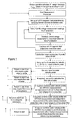
- FIG. 1 depicts a flow chart showing the operational steps of an embodiment of an electromagnetic flow mete according to the invention
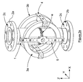
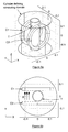
- FIG. 2 a depicts a perspective view of a further embodiment of an electromagnetic flow meter according to the invention.
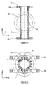
- FIG. 2 b depicts a schematic cross-sectional view of the flow meter of FIG. 2 a;
- FIG. 2 c depicts a schematic top view of the flow meter of FIG. 2 a;
- FIG. 2 d depicts a schematic view of the electrode configuration and pixels of the flow cross-section of the flow meter of FIG. 2 a;
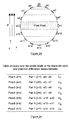
- FIG. 2 e is a table showing how the pixels relate to the pairs of electrodes and potential different measurements for the flow meter of FIG. 2 a;
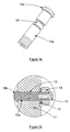
- FIG. 3 a depicts a perspective view of an embodiment of a voltage detecting electrode according to the invention
- FIG. 3 b depicts the electrode of FIG. 3 a mounted in the wall of the flow tube of an electromagnetic flow meter
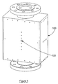
- FIG. 4 depicts a housing enclosing at least part of the flow meter of FIG. 2 a;
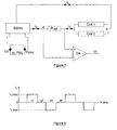
- FIG. 5 depicts a combined coil excitation and temperature compensation circuit for an electromagnetic flow meter according to the invention
- FIG. 6 depicts a graph showing how the coil current varies with time
- FIG. 7 depicts a voltage measuring circuit for collating the voltage measured between the jth pair of electrodes and a control circuit for eliminating the effects of an unwanted voltage U o .
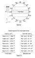
- FIG. 8 a depicts a 3-dimensional schematic diagram of an example of a flow meter where the flow tube defines the computing domain
- FIG. 8 b depicts a 2-dimensional schematic diagram of the flow meter of FIG. 8 a
- FIG. 9 depicts a schematic view of the flow pixels in the flow meter of FIG. 8 a;
- FIG. 10 depicts a table that lists the geometries of the flow meter of FIG. 8 a;
- FIG. 11 a depicts a distribution of the Lorentz force per unit volume when simulating a flow meter to determine weight values
- FIG. 11 b depicts the electrical potential on the z-plane when simulating a flow meter to determine weight values
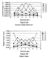
- FIG. 12 a depicts the induced voltages when simulating a flow meter to determine weight values
- FIG. 12 b depicts the weight values calculated from the induced voltages of FIG. 12 a
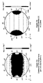
- FIG. 13 a depicts a distribution of the Lorentz force per unit volume on a conducting fluid with a uniform flow profile
- FIG. 13 b depicts the electrical potential on the z-plane of the conducting fluid of FIG. 13 a;
- FIG. 14 a depicts a distribution of the Lorentz force per unit volume on a conducting fluid with a non-uniform flow profile
- FIG. 14 b depicts the electrical potential on the z-plane of the conducting fluid of FIG. 14 a;
- FIG. 15 a depicts the axial velocity profile of a conducting fluid with a uniform flow profile
- FIG. 15 b depicts the axial velocity profile of a conducting fluid with a non-uniform flow profile
- FIG. 16 depicts an electrode potential rotational pattern showing the resultant effective sensing region and centre of action for an 8 electrode system of an ICC measuring means.
- the invention relates to an electromagnetic flow meter and method for monitoring the flow of a conducting fluid.
- the flow meter and method determine the axial velocity profile of a conducting fluid.
- the conducting fluid may be a conducting single phase fluid or a conducting continuous phase of a multiphase fluid.
- the conducting fluid may have a uniform flow profile or a non-uniform flow profile.
- the flow meter comprises a flow tube, a means for generating a magnetic field across the flow tube cross-section, an array of voltage detection electrodes circumferentially arranged around the flow tube and processing means for determining the axial velocity profile of a conducting fluid.
- the flow tube is a pipe along which fluid can flow when the flow meter is in use.
- the fluid may be a conducting single phase fluid or a multiphase fluid comprising a conducting continuous phase and at least one dispersed phase.
- the means for generating a magnetic field is configured to generate a magnetic field across the flow tube cross-section so that a voltage is induced in the conducting fluid as it flows through the flow tube.
- the means for generating a magnetic field may successively generate multiple magnetic fields, each magnetic field having a different magnetic flux density distribution.
- Each magnetic flux density distribution may be referred to as a magnetic field projection.
- the number of projections generated is P, whereby P ⁇ 1.
- the flow meter comprises an array of E electrodes.
- the electrodes are circumferentially mounted on an internal surface of the flow tube so as to detect the induced voltage between various points on the circumference of the flow tube.
- the electrodes are configured so as to divide the flow cross-section into pixels (discrete regions) and to measure the local induced voltage in each pixel.
- the electrodes are able to measure the induced voltage of the conducting fluid in N pixels (discrete regions) in the flow cross-section.
- the processing means is configured to determine the axial velocity profile of the conducting fluid using the measured induced voltages and predetermined weight functions.
- the charged particles of the conducting fluid experience a Lorentz force as they move in the magnetic field.
- the Lorentz force acts in a direction perpendicular to both the conducting fluid's motion and the applied magnetic field.
- the expression (v ⁇ B) represents the Lorentz force induced by the fluid motion, whereas E is principally due to charges distributed in and around the fluid.
- a i represents the cross sectional area of the i th of N pixels into which the flow cross section is divided
- v i is the mean axial flow velocity in the i th pixel
- U j is the j th of N potential difference measurements made at the boundary of the flow
- the term w is a so called weight value which relates the flow velocity in the i th pixel to the j th potential difference measurement
- a is the internal pipe radius
- B is the mean magnetic flux density in the flow cross section.
- the local axial velocity of the conducting fluid in each of the N pixels can be determined from predetermined weight values w ij and N potential difference measurements U j made on the boundary of the flow using the electrodes.
- Equation 3 The N independent equations arising from equation 3 can be expressed by the following matrix equation:
- V is a single column matrix containing the pixel velocities v i
- W is a square matrix containing the relevant weight values w ij
- A is a square matrix containing information on the pixel areas A i
- U is a single column matrix containing the measured potential differences U j .
- equation 4 can be solved giving:
- the flow meter can determine the axial velocity profile of the conducting fluid by dividing the flow cross section into N pixels and using equation 5 to derive the axial flow velocity in each of the N pixels.
- the accuracy of the flow meter is at least partially determined by its spatial resolution (i.e. the number of pixels, N) and thereby the number of potential difference measurements that can be taken. Since the number of electrodes is restricted by the circumferential size of the flow tube, the accuracy of the flow may thereby be improved by increasing the number of magnetic flux density distributions P.
- the N independent potential difference measurements can be related to the unknown axial flow velocity v i in each of N discrete regions, or pixels, in the flow cross section by N independent equations of the form
- U j,p is the j th (of M) independent potential difference made using the p th (of P) projections
- a i is the area of the i th (of N) pixels
- w i,j,p is a weight value relating the flow velocity in the i th pixel to the j th potential difference measurement using the p th magnetic field projection
- B P is the mean flux density in the flow cross section associated with the p th projection
- a is the internal radius of the flow tube.
- R B ⁇ U 2 ⁇ ⁇ ⁇ a ⁇ WAV ( 7 )
- U is an (N ⁇ 1) matrix containing the measured potential differences
- W is an (N ⁇ N) matrix containing the known weight values
- A is an (N ⁇ N) matrix containing information on the known pixel cross sectional areas
- R B is an (N ⁇ N) matrix containing information on the reciprocals of the known mean flux densities in the flow cross section (associated with each of the P magnetic field projections)
- V is an (N ⁇ 1) matrix containing the unknown axial flow velocities in the N pixels.
- equation 7 can be solved giving
- the flow meter can determine the axial velocity profile of the conducting fluid by dividing the flow cross section into N pixels and using equation 7 to derive the axial flow velocity in each of the N pixels.
- R B [ 1 ⁇ / ⁇ B _ 1 0 ⁇ 0 0 0 1 ⁇ / ⁇ B _ 1 ⁇ 0 0 ⁇ ⁇ ⁇ ⁇ ⁇ 0 0 ⁇ 1 ⁇ / ⁇ B _ P 0 0 0 ⁇ 0 1 / B _ P ] ( A2 )
- W [ w 1 , 1 , 1 w 2 , 1 , 1 ⁇ w N , 1 , 1 w 1 , 2 , 1 w 2 , 2 , 1 ⁇ w N , 2 , 1 ⁇ ⁇ ⁇ w 1 , M , P w 2 , M , P ⁇ w N , M , P ] ( A3 )
- A [ A 1 0 ⁇ 0 0 A 2 ⁇ 0 ⁇ ⁇ ⁇ ⁇ 0 0 ⁇ A N ] ( A4 )
- V [ v 1 v 2 ⁇ v N ] ( A5 )
- the flow meter calculates the mean velocity of the conducting fluid in each pixel.
- the flow meter calculates the simple mean velocity of the conducting continuous phase which is calculated in each pixel. By simple mean it is implied that the calculated velocity is not weighted by the concentration, or local volume fraction, of the conducting continuous phase in the pixel.
- the axial velocity of the conducting fluid in each of the N pixels is determined using predetermined weight values w ij , w i,j,p .
- the weight values represent the relative contribution of the fluid flow at a particular spatial location in the flow cross section to the measured potential difference.
- N 2 weight values are required. These weight values are calculated, from solutions of Maxwell's equations of electromagnetism. These N 2 weight values are dependent upon the geometry of the electromagnetic flow meter, its materials of construction and also upon the magnetic field projections that are employed. The weight values need only be calculated once, prior to using the flow meter device. An example of how weight values can be calculated is described below.
- the flow meter and method may determine the volumetric flow rate of the conducting fluid.
- the volumetric flow rate Q c of the conducting single phase fluid can be calculated from the determined axial velocity profile as follows;
- the volumetric flow rate of the conducting continuous phase Q c can be determined providing the local concentration distribution (also known as the local volume fraction distribution) of the conducting continuous phase ⁇ c in the flow cross section is known.
- volumetric flow rate of the conducting continuous phase Q c can be calculated using the following equation:
- volumetric flow rate of the conducting continuous phase Q c can be calculated using the following equation:
- the flow meter preferably comprises means for measuring the local volume fraction distribution of the conducting continuous phase.
- the flow meter may comprise means for measuring the local volume fraction distribution using the well known technique of Electrical Resistance Tomography (ERT).
- ERT Electrical Resistance Tomography
- the flow meter may comprise means for measuring the local volume faction distribution using an impedance cross correlation technique (ICC).
- ICC impedance cross correlation technique
- the flow meter and method may also monitor the flow of the one or more dispersed phases of the multiphase fluid. For example, the flow meter and method may determine the local velocity of a dispersed phase in the flow cross section v d and optionally the volumetric flow rate of a dispersed phase Q d .
- the flow meter may comprise means for measuring the local velocity of the dispersed phase using an impedance cross correlation technique (ICC).
- ICC impedance cross correlation technique
- An example of flow meter comprising means for measuring the local velocity of the dispersed phase using an impedance cross correlation technique is described below.
- the volumetric flow rate of a dispersed phase can be determined providing the local concentration distribution (also known as the local volume fraction distribution) of the dispersed phase ⁇ d in the flow cross section is also known.
- the flow meter may comprise means for measuring the local volume fraction distribution of the dispersed phase ⁇ d using an impedance cross correlation technique).
- volumetric flow rate of the dispersed phase Q d can be calculated using the following equation:
- the flow meter may also comprise density measuring means for determining the mean density of a multiphase fluid.
- the flow meter and method can be used to make flow rate measurements of a conducting fluid in partially filled or partially blocked pipes, provided that a minimum of two electrodes are immersed in that part of the cross section of the pipe where flow still occurs.
- FIG. 1 depicts a flow diagram that shows the operational steps of an example of a flow meter and method according to the present invention.
- the conducting fluid is water:
- the flow meter comprises a means for generating a magnetic field across the flow tube cross-section, an array of voltage detection electrodes circumferentially arranged around the flow tube and processing means for determining the flow characteristics of the conducting fluid.
- the flow tube is a pipe along which fluid may flow when the flow meter is in use.
- the fluid may be a conducting single phase fluid or a multiphase fluid comprising a conducting continuous phase and at least one dispersed phase.
- the flow tube preferably comprises a body formed from a non-electrically conducting material, such as PTFE.
- the flow tube may comprise an outer body portion formed from a low magnetic permeability material and an inner body portion (e.g. a liner) formed from a non-electrically conducting material, thereby ensuring the electrodes are electrically isolated from each other.
- the flow tube may comprise an inner body portion (e.g. an annular liner) that is formed from a material having a conductivity that is at least similar to that of the conducting phase flow and deployed between the electrodes and the flow in order to improve the uniformity of weight function values.
- the flow tube may have any suitable diameter and length.
- the diameter and length of the flow tube may be selected according to the type of fluid, volume of fluid and/or location of the flow tube.
- an electrically conducting single phase fluid may flow through the flow tube, such as water.
- a multiphase fluid having an electrically conducting continuous phase and one or more dispersed phases may flow along the flow tube.
- Examples of a multiphase fluid include solids-in-water flows such as sludges and slurries, oil-in-water flows, gas-in-water flows, and oils and gas-in-water flows.
- FIGS. 2 a - 2 d depict an embodiment of a flow meter according to the first aspect of the invention whereby the flow tube ( 1 ) is a PTFE pipe with an internal diameter of approximately 80 mm, an external diameter of approximately 110 mm and a length of approximately 410 mm.
- the flow meter may comprise a flange arranged at one or both ends of the flow tube.
- the flange may be configured so as to allow the flow meter to be coupled to a further apparatus, such as a pipe.
- the flange may comprise one or more apertures to receive securing means (e.g. bolts, screws, clips etc) suitable for securing the flow meter to a further apparatus.
- the electromagnetic flow meter comprises a first flange ( 2 a ) arranged at a first end of the flow tube and a second flange ( 2 b ) arranged at a second end of the flow tube.
- the flanges have a diameter of approximately 203 mm and a thickness of approximately 24 mm.
- the flanges are configured so that the flow meter can be connected to external pipe work.
- Each flange comprises a plurality of bolt holes ( 2 c ) with an internal diameter of approximately 16 mm.
- the means for generating a magnetic field in the flow meter is configured to generate a magnetic field so that a voltage is induced across the conducting fluid as it flows through the flow tube. As shown in FIGS. 2 a - 2 d , the means for generating a magnetic field generate a magnetic field that is orthogonal to both the direction of the flowing fluid and plane of the array of electrodes so that the potential difference at the boundary of the flow tube can be detected by the electrodes.
- the means for generating a magnetic field may generate a generally uniform magnetic field across the flow tube.
- the means for generating a magnetic field may generate a non-uniform magnetic field across the flow tube.
- the means for generating a magnetic field may be configured to generate a non-uniform magnetic field across each pixel (discrete region) of the flow tube cross-section.
- the non-uniform magnetic field may be applied to help distinguish between different axisymmetric or non-axisymmetric velocity profiles.
- the means for generating a magnetic field comprises any suitable electromagnetic means for generating a magnetic field.
- the means for generating a magnetic field may comprise a Helmholtz coil mounted around the periphery of the flow tube.
- the Helmholtz coil comprises a pair of identical coils ( 3 a , 3 b ) arranged symmetrically on opposing sides of the flow tube as shown in FIGS. 2 a to 2 d .
- the Helmholtz coil may be securely mounted to the flow tube using coil supports/stiffeners ( 4 ) and coil mounting brackets ( 5 ).
- the Helmholtz coil may comprise any suitable size and number of turns.
- the coils may have a mean diameter that is approximately twice the mean coil separation distance.
- the coils of the Helmholtz coil are approximately 30 mm thick, approximately 29 mm wide, have an internal diameter of approximately 202 mm, have an external diameter of approximately 260 mm, comprise approximately 1024 turns of 0.776 mm diameter wire and have an approximately 5 AMP capacity.
- the means for generating a magnetic field may successively generate multiple magnetic fields, each magnetic field having, a different magnetic flux density distribution.
- Each magnetic flux density distribution may be referred to as a magnetic field projection.
- the number of projections generated is P, whereby P ⁇ 1.
- Each projection may be consecutively applied for a short time interval.
- the magnetic flux density distribution across the flow tube is dependent on the magnitude and direction of the electrical current in the Helmholtz coil.
- different magnetic flux density distributions may be generated by varying the magnitude and/or direction of the electrical currents supplied to the Helmholtz coil.
- the different magnetic flux density distributions may be generated by arranging multiple pairs of Helmholtz coils in different planes around the flow tube.
- the means for generating a magnetic field preferably generates a magnetic field having a rectangular waveform so as to minimise the effects of electrolysis at the electrodes.
- the means for generating a magnetic field may generate a rectangular waveform magnetic field alternating between +/ ⁇ 40 Gauss.
- the Helmholtz coil is configured such that current flows through both coils in the same direction and each coil carries an equal amount of electric current.
- the Helmholtz coil generates a generally single and uniform magnetic flux density distribution in the flow cross section.
- the magnitude of the magnetic flux density in the y direction is relatively constant and the mean value B of the magnitude of the y component of the magnetic flux density in the flow cross section is 7.996 Gauss (7.996 ⁇ 10 ⁇ 4 T).
- the flow meter comprises an array of E electrodes.
- the electrodes are circumferentially mounted on an internal surface of the flow tube so as to detect the induced voltage at various points on the internal circumference of the flow tube.
- the electrodes are arranged as opposing pairs around the circumference of the flow tube so as divide the flow cross-section into pixels (discrete regions) and to measure the local induced voltage in each of the pixels.
- the electrodes are able to measure the induced voltage of the conducting fluid in N pixels (discrete regions) in the flow cross section.
- the pixels may be parallel, elongate regions extending between opposing sides of the flow tube.
- the pixels can be of any shape or size provided that, in total, they entirely cover the (normally circular) cross section of the flow tube.
- the electromagnetic flow meter may comprise any suitable number of electrodes.
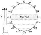
- the electrodes are placed at angular intervals of 22.5 degrees on the flow pipe boundary.
- the electrodes are denotated e 1 , e 2 , etc, with electrodes e 5 at the top of the flow cross section and electrode e 13 at the bottom of the flow cross section.
- the electrodes are configured such that the flow cross-section is divided into seven pixels.
- the geometry of these seven pixels is chosen such that the chords joining seven pairs of electrodes are located at the geometric centres (in the y direction) of the pixels.
- the fluid pixels are categorized as pixel 1 at the top of the flow cross section to pixel 7 at the bottom of the flow cross section.
- Seven potential difference measurements can be made between the seven electrode pairs. Since the jth potential difference measurement U j is made between the jth electrode pair, the potential difference measurements are notated U 1 , U 2 etc in the table depicted in FIG. 2 e .
- the local magnetic flux density B is perpendicular to both the flow direction and to the chords joining the electrode pairs.
- the electrodes may be made from a low magnetic permeability material (e.g. stainless steel or brass) if the flow tube comprises a non-electrically conducting pipe wall.
- the electrodes are configured to be electrically insulated from the outer metal wall. This may be achieved by enclosing each of the electrodes in a non-conducting liner.
- FIG. 3 a depicts an embodiment of an electrode ( 10 ) for an electromagnetic flow meter when the flow tube comprises a non-electrically conducting body.
- the electrode comprises an elongate body portion ( 10 a ) and a head portion ( 10 b ).
- the electrode is mounted on the flow tube such that the head portion is arranged on the inner side of the flow tube so it can form a contact with the flowing fluid and the body portion extends through an aperture in the wall of the flow tube ( 11 ) and protrudes beyond the flow tube.
- An O-ring seal ( 12 ) is arranged between the body portion and the internal surface of the aperture so as to form a seal between the electrode and the flow tube.
- the O-ring seal may be mounted in a circumferential groove formed on the body portion of the electrode.
- the electrode may be secured to the flow tube using any suitable securing means, such as a retaining nut ( 13 ).
- a rubber washer ( 14 ) may be arranged between the retaining nut and the external surface of the flow tube.
- the electrode may be electrically connected to an electrical cable using an suitable coupling means, such as a screw connector ( 15 ).
- FIG. 4 depicts an embodiment of a flow meter whereby the flow tube and array of electrodes may be located (encased) in a housing ( 100 ).
- the housing preferably acts as a Faraday cage so as to prevent external electrical fields from interfering with the induced voltages measure at the electrodes.
- the housing preferably acts as a magnetic shield so as to prevent external magnetic fields from interfering with the operation of the flow meter and also prevent “leakage” of the magnetic field generated by the means for generating a magnetic field into the surrounding environment.
- the housing may comprise an aperture ( 101 ) through which an electrical cable may extend from the electrode array to the processing means.
- the flow meter comprises processing means for determining at least the axial velocity profile of the conducting fluid.
- the processing means is configured to determine the axial velocity profile by calculating the axial velocity of the conducting fluid in each pixel of the flow cross-section.
- the processing means comprises means to calculate the axial velocity of the conducting fluid in each pixel of the flow cross section using an inverted matrix.
- the processing means comprises means to derive the axial velocity of the conducting fluid in each pixel of the flow cross section using equation 5 when a single magnetic field projection is applied.
- the processing means comprises means to derive the axial velocity of the conducting fluid in each pixel of the flow cross section using equation 8 when multiple magnetic field projections are applied.
- the processing means may comprise means to determine the weight function values of the pixel prior to determining the axial velocity profile of the conducting fluid.
- the processing means is preferably further configured to determine the volumetric flow rate of the conducting fluid.
- the processing means may comprise means to calculate the volumetric flow rate using the axial velocity profile of the conducting fluid. More specifically, the processing means may comprise means to calculate the volumetric flow rate using equation 9 when the conducting fluid is a conducting single phase fluid.
- the processing means may be configured to derive the volumetric flow rate using the axial velocity profile and local volume fraction distribution of the conducting fluid.
- the processing means may comprise means for measuring the local volume fraction distribution of the conducting fluid using an electrical resistance tomography technique or an impedance cross correlation technique.
- the processing means may be configured to determine flow characteristics of each phase of a multiphase fluid.
- the processing means may be configured to determined the axial velocity profiles, local volume fraction distributions and/or volumetric flow rates of the conducting continuous phase and the at least one dispersed phase.
- the processing means may be configured to control the operation of the flow meter.
- the processing means may be a microcontroller.
- a suitable microcontroller is the Microrobotics VM-1 microcontroller.
- the processing means may comprise any suitable hardware, operating systems and/or software.
- the processing means may comprise display means for displaying the calculated flow characteristics of the fluid.
- the processing means may be configured to control the operation of the means for generating the magnetic field.
- the processing means may comprise means for controlling the flow of current to the means for generating a magnetic field (e.g. the Helmholtz coil).
- the means for controlling the flow of current supplies a sinusoidal current to the Helmholtz coil to achieve a time varying magnetic field.
- the means for controlling the flow of current (such as the coil excitation circuit shown in FIG. 5 ) may apply a hybrid square wave current (as shown in FIG. 6 ) to the Helmholtz coil (Coil 1 , Coil 2 ) to achieve a time varying magnetic field.
- the hybrid square wave current may complete a cycle in approximately 0.5 seconds or less.
- the dc power supply unit (dc PSU) is connected to a network of solid state relays.
- the solid state relay network (SSRN) is controlled by the processing means in such a way that at any instant in time the voltages applied at points ‘a’ and ‘b’ in FIG. 5 are as per the table below.
- the two coils of the Helmholtz coil (Coil 1 , Coil 2 ) are closely matched and the resistance R c of each coil has a known value of R c,15 when the coils are at a temperature of 15° C.
- the ambient temperature variations and the heating of the coils due to the coil current cause the value of R c , and thereby i c,max , to vary with time.
- the flow induced voltages U j from which the flow velocity profile is reconstructed are proportional to B max —the maximum value of the mean magnetic flux density in the flow cross section.
- the processing means preferably comprises a temperature compensating circuit to determine i c,max and thereby B max .
- FIG. 5 depicts an example of a temperature compensating circuit whereby the coil current i c is passed through the high tolerance reference resistor with a known resistance R ref .
- the reference resistor has a very low temperature coefficient.
- a voltage U r appears across R ref and is fed to the processing means via a differential amplifier (DA).
- DA differential amplifier
- the processing means may be further configured to collate the potential difference measurements in each pixel.
- the processing means may comprise means for collating the potential difference between each pair of electrodes.
- FIG. 7 depicts an example of a voltage measuring circuit suitable for collating the potential difference measurements between a pair of electrodes.
- a voltage measurement is being made between the jth pair of electrodes.
- a circuit such as that shown in FIG. 7 is necessary for each pair of electrodes between which is required to make a voltage measurement.
- 15 such circuits are required for a flow meter comprising 16 electrodes and requiring 15 voltage measurements.
- a voltage U j necessary for reconstructing the velocity profile is extracted from U* j at the processing means sing appropriate signal processing techniques.
- U* j is also a rapidly varying signal.
- the amplitude of U* j is only a few millivolts and so before being sampled by the analogue to digital converter in the processing means it must be amplified by a high gain differential amplifier (HGA) which has gain A, where A is typically equal to 1000.
- HGA high gain differential amplifier
- a voltage follower (VF) and HPF) are used to condition the signals from the electrodes prior to being passed to HGA.
- the high pass filters are used to eliminate a very large dc offset which can appear on each electrode due to the effects of polarisation and accumulation of static charges.
- the output voltage U x,j from the high gain amplifier (HGA) is fed to the processing means.
- the differential voltage at the input to HGA consists of the sum of U* j and a residual, unwanted slowly varying dc voltage U 0 due to the effects of polarisation and accumulation of static charges at the electrodes.
- U 0 is generally larger than the amplitude of U* j . If the effects of U 0 are not eliminated then the voltage U x,j at point x in FIG.
- the processing means preferably comprises a control circuit to compensate for the effects of U 0 .
- FIG. 7 depicts an example of a control circuit that is configured to compensate for the effects of U 0 by applying a suitable offset (or reference) voltage to HGA at point y.
- the control circuit depicted in FIG. 7 comprises a low pass filter (LPF), a differential amplifier (DA), a set point adjustor (SPA) and an integrator (INT).
- LPF low pass filter
- DA differential amplifier
- SPA set point adjustor
- INT integrator
- the processing means comprises the coil excitation circuit, temperature compensation circuit, voltage measurement circuit and control circuit as depicted in FIGS. 5 and 7
- the operation of the solid state relay network to control the current i c applied to the coils can be as follows:
- the values of U j given by equation 21 may be calculated for a single coil current cycle or they may be averaged using the processing means over G coil current cycles where G may take user specified values of, for example, 1, 2, 5 etc.
- the required value of G may be entered into the processing means software by the user via a touch screen display.
- the mean magnetic flux density term B used in the calculation of the pixel velocities is set equal to B max in the processing means software.
- B B max (23)
- V ⁇ ⁇ ⁇ a 2 ⁇ B _ ⁇ [ WA ] - 1 ⁇ U ( 24 )
- V is the matrix containing the calculated pixel velocities v i
- w is a matrix of the electromagnetic flow meter weight functions w ij which are stored in the processing means software
- A is a matrix of the pixel areas A i which are stored in the processing means software
- U is a matrix constructed from the measured potential differences U j given by equation 20.
- the term a in equation 24 is the internal radius of the flow cross section of the flow meter body. [Note that for a single phase flow v i is the conducting fluid velocity in the i th pixel. For a multiphase flow v i is the velocity of the conducting continuous phase in that pixel].
- the values of the pixel velocities v i may be displayed on the processing means display either graphically or ‘alphanumerically’.
- the total liquid flow rate Q c is calculated and displayed by the processing means using equation 25 below.
- the processing means preferably operates continuously, updating the display of the pixel velocities v i and of Q c after every G coil current cycles
- the following description relates to an embodiment of an electromagnetic flow meter according to the present invention.
- the description describes how the weight function values of each pixel can be calculated for the flow meter.
- the description describes how the volumetric flow rate of a conducting single phase fluid (water) may be determined by the flow meter from the weight values and boundary voltage measurements.
- the description describes how the volumetric flow rate of a conducting single phase fluid having a uniform velocity profile across the cross-section of the flow tube may be determined using the flow meter.
- the description also describes how the volumetric flow rate of a conducting fluid having a non-uniform velocity profile across the cross-section of the flow tube may be determined using the flow meter.
- This particular flow meter consists of a PTFE (polytetrafluoroethylene) flow pipe (T) mounted within Helmholtz coils (C 1 , C 2 ).
- the inner diameter of the flow pipe is 0.08 m
- the outer diameter is 0.09 m
- its axial length is 0.3 m.
- the inner and outer diameters of the two coils are 0.2048 m and 0.2550 m respectively.
- a cylindrical domain with a diameter of 0.32 m and a length of 0.32 m represents the boundary of the computing domain (refer to FIGS. 8 a and 8 b ).
- Sixteen electrodes are placed at angular intervals of 22.5 degrees on the flow pipe boundary (refer to FIG. 9 ) the electrodes being denoted e 1 , e 2 etc, with electrode e 5 at the top of the flow cross section and electrode e 13 at the bottom of the flow cross section.
- the flow cross section is divided into seven pixels. The geometry of these seven pixels is chosen such that the chords joining seven pairs of electrodes are located at the geometric centres (in the y direction) of the pixels (refer to FIG. 9 ).
- the fluid pixels are categorized as pixel 1 at the top of the flow cross section to pixel 7 at the bottom of the flow cross section.
- the pixel areas A i are shown in the table depicted in FIG. 10 .
- Seven potential difference measurements can be made between the seven electrode pairs as shown in the table of FIG. 10 (the j th potential difference measurement U 1 was made between the j th electrode pair shown in the table of FIG. 10 1 ).
- the local magnetic flux density B is perpendicular to both the flow direction and to the chords joining the electrode pairs.
- a Helmholtz coil is used to produce a nearly uniform local magnetic flux density distribution.
- the Helmholtz coil consists of two identical circular electromagnetic coils. In the flow meter design these coils are placed symmetrically on each side of the PTFE flow pipe as shown in FIGS. 8 a and 8 b .
- the system is designed such that the current flows through both coils in the same direction and each coil carries an equal amount of electric current giving rise to a relatively uniform magnetic flux density distribution in the flow cross section.
- the magnitude of the magnetic flux density in the y direction is relatively constant and has a maximum value of 7.757 ⁇ 10 ⁇ 4 T and minimum value of 8.044 ⁇ 10 ⁇ 4 T in the flow cross section.
- the mean value B of the magnitude of the y component of the magnetic flux density in the flow cross section is 7.996 ⁇ 10 ⁇ 4 T (7.996 gauss).
- the weight values w ij of each pixel relate to the axial velocity v i in the i th pixel to the j th potential difference measurement U j .
- the weight function values can be determined by simulating the flow meter using COMSOL Multiphysics software. As part of the simulation process, the flow channel is divided into seven pixels as described above (refer to FIG. 9 ). The condition of the simulation is that the fluid in the pixel for which weight values are to be calculated is given a flow velocity of greater than zero in the z direction whilst the remaining pixels all have zero fluid velocity.
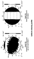
- FIG. 11 a and 11 b show the distribution of the Lorentz forces and the induced electrical potentials when the fluid in pixel 4 has an imposed velocity in the z direction while the fluid in the remaining fluid pixels is at rest.
- FIG. 11( a ) illustrates the Lorentz force distribution arising from the imposed velocity in pixel 4 .
- the magnetic field interacts with the charges carried in the water via these Lorentz forces causing the separation of charged ions (positive and negative) and giving rise to the electrical potential distribution shown in FIG. 11( b ).
- the arrows shown in FIG. 11( a ) also represent the direction of the local induced current density and it can be seen that for the (highly contrived) case in which flow occurs in pixel 4 only there is circulation of the electric current.
- FIG. 12( a ) shows the induced voltages plotted against electrode pairs for all of the seven simulations. [Note that the very large simulated pixel velocity of 500 ms ⁇ 1 was used to improve the accuracy of the weight values calculated using COMSOL].
- FIG. 12( b ) shows the 49 weight values calculated from the induced voltages given in FIG. 8( a ) by using equation 26.
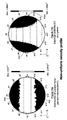
- FIGS. 13 a and 13 b shows the effect of a uniform velocity distribution of 50 ms ⁇ 1 in the flow cross section on the Lorentz force distribution and the electrical potential distribution.
- the conducting fluid may be a single phase flow or the conducting continuous phase of a multiphase flow.
- FIGS. 14 a and 14 b shows the effect of a non-uniform velocity distribution in the flow cross section on the Lorentz force distribution and the electrical potential distribution.
- the flow velocity v z in the z direction is given by the expression
- v 2 1 + ( y a ) ( 27 )
- y is the coordinate defined in FIGS. 14 a and 14 b and a is the internal pipe radius.
- This type of non-uniform velocity profile is non-axisymmetric and has a linear velocity distribution in the flow cross section.
- the non-uniform velocity profile can occur in single phase flows where flow is some how restricted (e.g. by a bend in the pipe or a partially opened valve.)
- this type of non-uniform velocity profile can occur in multiphase flows, for example, inclined multiphase flows.
- the relevant induced voltages U j for the uniform velocity profile and linear velocity profile were measured using the electrode pairs shown in the table of FIG. 10 . It should be noted that the electrical potential distribution for the uniform velocity profile and non-uniform velocity profile are entirely different from each other. For the uniform velocity distribution the induced voltages between pairs 1 , 2 and 3 are the same as for pairs 7 , 6 , and are respectively. For the non-uniform velocity profile the induced voltage between pair 1 is higher than that for pair 7 . Similarly the induced voltages between pairs 2 and 3 are respectively higher than for pairs 6 and 5 . Moreover, for the non-uniform velocity profile the highest induced potential is between electrode pair 3 while the maximum induced voltage for the uniform velocity profile is between electrode pair 4 .
- the predetermined weight function values w ij and measured induced voltages are used to determine the mean velocity v i in each pixel.
- the method can be expressed simply by the following matrix equation
- V ⁇ ⁇ ⁇ a 2 ⁇ B _ ⁇ [ WA ] - 1 ⁇ U ( 5 ) in which V is a single column matrix containing the pixel velocities v i , W is a square matrix containing the relevant weight values w ij , A is a square matrix containing information on the pixel areas A i and U is a single column matrix containing the calculated potential differences U j for a given imposed velocity profile.
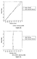
- FIGS. 15( a ) and 15 ( b ) The two velocity profiles of water as determined by the flow meter are shown in FIGS. 15( a ) and 15 ( b ). Also shown in FIGS. 15( a ) and 15 ( b ) are the imposed/reference velocity profiles that were measured using other detection means.
- the reference velocity profiles may be determined for example by using a laser Doppler anemometry device, hot wire anemometry device or a pitot-static tube.
- FIGS. 15 a and 15 b show that the velocity profiles determined by the flow meter have excellent agreement with the reference velocity profiles for both the uniform and non-uniform velocity profiles.
- FIG. 15( a ) shows that for the uniform velocity profile the maximum (most overestimated) and minimum (most under estimated) errors occur in pixel 1 (+4.565%) and pixel 5 ( ⁇ 3.33%) respectively. The most accurate velocity is in pixel 4 with an error of only 0.722%.
- the non-uniform velocity profile has maximum and minimum errors in pixels 2 and 7 respectively.
- the most accurate velocities for the non-uniform velocity profile are in pixels 3 and 6 with errors of +0.912% and ⁇ 0.797% respectively.
- the total volumetric flow rate Q w of the water can be calculated from the determined velocity profile as follows;
- Q wiu the true volumetric flow rate associated with the imposed (reference) uniform velocity profile
- Q wru the volumetric flow rate associated with the calculated (determined) uniform velocity profile
- Q wiu is calculated to be 2.509 ⁇ 10 ⁇ 1 m 3 s ⁇ 1 and Q wru is found to be 2.503 ⁇ 10 ⁇ 1 m 3 s ⁇ 1 . There is thus an error of only ⁇ 0.238% in the total volumetric flow rate obtained from the calculated uniform velocity profile.
- the following description relates to a flow meter that is suitable for monitoring the flow of a two phase fluid.
- the fluid comprises a conducting continuous phase and a dispersed phase.
- the flow meter is suitable for determining the axial velocity profile of the conducting continuous phase as discussed above.
- the flow meter further comprises an impedance cross correlation measuring means (ICC) for measuring the distribution of the local velocity v d of the dispersed phase in the flow cross section.
- the ICC is also able to measure the distribution of the local volume fractions of the dispersed and continuous phase ( ⁇ d and ⁇ c respectively) in the flow cross section.
- the ICC measuring means consists of two arrays of ⁇ electrodes denoted array ‘ ⁇ ’ and array ‘ ⁇ tilde over (B) ⁇ ’ spaced uniformly around the internal circumference of the pipe.
- One of these electrode arrays may, if required, be the same as the electrode array used in the flow meter for determining the axial flow velocity of the conducting continuous phase.
- ⁇ is typically equal to 8 or 16.
- the axial separation L of the arrays is typically 50 mm.
- the distributions of the local volume fractions ⁇ d and ⁇ c are measured using one of the arrays only (e.g. array ⁇ tilde over (B) ⁇ ).
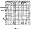
- a sequence I of electrical potentials is applied to the electrodes in array ⁇ tilde over (B) ⁇ , starting at electrode ‘Elec 1 ’ ( FIG. 16 ), giving rise to an Electrode Potential Rotational Pattern (EPRP) denoted I 1 .
- EPRP Electrode Potential Rotational Pattern
- the potential applied to an electrode may be ‘excitation’ (denoted V + ), ‘virtual earth’ (denoted ve) or ‘true earth’ (denoted E).
- E ‘true earth’
- the ‘Effective Sensing Region’ R I,1 has a ‘Centre of Action’ denoted C I,1 with precisely defined coordinates. If the conductivity ⁇ w of the conducting continuous phase is known then the ‘local’ dispersed phase volume fraction ⁇ d in R I,1 , (and hence at C I,1 ) can be determined from ⁇ m using the Maxwell relationship for mixtures of conducting materials
- ⁇ d 2 ⁇ ⁇ w - 2 ⁇ ⁇ m ⁇ m + 2 ⁇ ⁇ w ( a3 )
- the new EPRP is I 2 and the new effective sensing region is R I,2 which has the same shape as R I,1 but which is rotated by
- R I,2 The centre of action of R I,2 is denoted C I,2 and the local volume fractions ⁇ d and ⁇ c of the dispersed and continuous phases at C I,2 can be determined as described above.
- sequence II e.g. ve, V + , ve, E, E, E, E, E.
- sequence II e.g. V + , ve, E, E, E, E, E.
- the local dispersed phase velocity v d at C I,1 is then given by
- Measurements of ⁇ d , ⁇ c and v d using the ICC device are calculated using the same processing means as that used in the flow meter for determining the axial velocity profile.
- DP-ERT Dual-Plane Electrical Resistance Tomography
- the following description relates to a flow meter that is suitable for monitoring the flow of each phase of a three phase fluid.
- the fluid comprises a conducting continuous phase and two dispersed phases.
- the flow meter further comprises an impedance cross correlation measuring means (ICC) and a density measuring means (DM) so as to create a three phase flow meter.
- ICC impedance cross correlation measuring means
- DM density measuring means
- the density meter could simply consist of a vertical section of pipe (of typical length 1 m) with pressure tapings separated by a vertical distance L DM .
- a differential pressure measurement ⁇ P DM made between the pressure tapings, compensated, for the effects of frictional pressure loss resulting from the motion of the multiphase mixture, enables the mean density ⁇ m of the multiphase to be measured using
- ⁇ m ⁇ ⁇ ⁇ P DM g ⁇ ⁇ ⁇ L DM ( b1 )
- ⁇ tilde over (g) ⁇ is the acceleration of gravity.
- a i is the area of the i th region (of N) into which the flow cross section is divided
- A is the total pipe cross sectional area
- ⁇ d ICC,i is the local volume fraction of the combined, non-conducting dispersed phases (oil and gas) in the i th region as measured by the ICC device.
- the mean volume fraction ⁇ o of the oil in the cross section can now be obtained using
- ⁇ o ( ⁇ m - ⁇ g ) - ⁇ w ⁇ ( ⁇ w - ⁇ g ) ⁇ o - ⁇ g ( b3 )
- ⁇ o , ⁇ w and ⁇ g respectively represent the densities of the oil, water and gas at the position of the three phase flow meter. It is necessary to calculate ⁇ g using simple, auxiliary measurements of the absolute pressure and absolute temperature of the multiphase mixture at the position of the multiphase flow meter.
- the volumetric flow rate Q w of the water can be obtained using
- the gas is not finely dispersed in the multiphase mixture in the way that the oil is finely dispersed in the water and so the mean gas velocity v g can be obtained as follows using the ICC device
- v g ICC,i is the local gas velocity, in the i th region into which the flow cross section is divided, as measured by the ICC device using the cross correlation technique described in the two phase flow meter.
Landscapes
- Physics & Mathematics (AREA)
- Fluid Mechanics (AREA)
- General Physics & Mathematics (AREA)
- Electromagnetism (AREA)
- Engineering & Computer Science (AREA)
- Power Engineering (AREA)
- Measuring Volume Flow (AREA)
Abstract
Description
j=σ(E+v×B) (1)
where σ is the local fluid conductivity, E is the local electric field in the stationary coordinate system, v is the local fluid velocity, and B is the local magnetic flux density. The expression (v×B) represents the Lorentz force induced by the fluid motion, whereas E is principally due to charges distributed in and around the fluid.
∇2 U=∇·(v×B) (2)
where v is the local fluid velocity and B is the local magnetic flux density.
where Ai represents the cross sectional area of the ith of N pixels into which the flow cross section is divided, vi is the mean axial flow velocity in the ith pixel, Uj is the jth of N potential difference measurements made at the boundary of the flow, the term w is a so called weight value which relates the flow velocity in the ith pixel to the jth potential difference measurement and a is the internal pipe radius and
in which V is a single column matrix containing the pixel velocities vi, W is a square matrix containing the relevant weight values wij, A is a square matrix containing information on the pixel areas Ai and U is a single column matrix containing the measured potential differences Uj.
Thus, when a single magnetic field projection is applied, the flow meter can determine the axial velocity profile of the conducting fluid by dividing the flow cross section into N pixels and using
where Uj,p is the jth (of M) independent potential difference made using the pth (of P) projections, Ai is the area of the ith (of N) pixels, wi,j,p is a weight value relating the flow velocity in the ith pixel to the jth potential difference measurement using the pth magnetic field projection,
where U is an (N×1) matrix containing the measured potential differences, W is an (N×N) matrix containing the known weight values, A is an (N×N) matrix containing information on the known pixel cross sectional areas, RB is an (N×N) matrix containing information on the reciprocals of the known mean flux densities in the flow cross section (associated with each of the P magnetic field projections) and V is an (N×1) matrix containing the unknown axial flow velocities in the N pixels.
Thus, when multiple magnetic field projections are applied, the flow meter can determine the axial velocity profile of the conducting fluid by dividing the flow cross section into N pixels and using
- (i) U is a (N×1) matrix where the term Uj,p represents the jth potential difference measurement associated with the pth magnetic field projection; (j=1 to M and p=1 to P).
- (ii) RB is an (N×N) diagonal matrix where
B p is the mean magnetic flux density in the flow cross section associated with the pth magnetic field projection; (p=1 to P).
- (iii) W is an (N×N) matrix where wi,j,p is the weight value relating the axial flow velocity in the ith pixel to the jth potential difference measurement associated with the pth magnetic field projection (i=1 to N, j=1 to M and p=1 to P).
- (iv) A is a (N×N) diagonal matrix where Ai is the cross sectional area of ith pixel; (i=1 to N).
- (v) V is a (N×1) matrix where vi is the axial flow velocity in the ith pixel; (i=1 to N).
in which Qc is the volumetric flow rate, Ai is the area of the ith(of N) pixel, and vi is the axial velocity in the ith pixel.
where vc is the local axial velocity in the flow cross section, αc is the local volume fraction distribution of the conducting continuous phase and A is the flow tube cross sectional area.
where Vi c is the velocity of the conducting continuous phase in the ith pixel into which the flow cross section is divided, αi c is the local volume fraction distribution of the conducting continuous phase in the ith pixel, and A i is the area of the ith pixel.
where vd is the local axial velocity in the flow cross section, αd is the local volume fraction distribution of the dispersed phase and A is the flow tube cross sectional area.
Q d=λd
where λd is the means volume fraction of the dispersed phase in the flow cross section as measured using an impedance cross correlation technique,
-
Step 1—Prior to starting the measuring procedure, the flow meter calculates the weight functions for each pixel. -
Step 2—On starting the measuring procedure, the flow meter generates a pth (of P) magnetic field projections so as to induce a voltage in the conducting fluid. -
Step -
Step 5—if multiple magnetic field projections are to be used, the flow meter repeatssteps 2 to 4 until P magnetic field projections have been applied. -
Step 6—the flow meter determine the total number of pixels/potential difference measurements. -
Step 7—the flow meter calculates the axial velocity of the conducting fluid in each of thepixels using equation 5 if P=1 orequation 8 if P>1 and optionally the flow meter stops/returns to the start if only the axial velocity profile of a conducting fluid is required. -
Optional Step 8—when monitoring a conducting single phase fluid, the flow meter may calculate the volumetric flow rate of the conducting fluid using equation 9. - Optional Step 9—when monitoring a two phase fluid, the flow meter may combine the axial velocity profile of a conducting continuous phase with local volume fraction measurements of the conducting continuous phase and dispersed phase and also the local axial velocity of the dispersed phase (measured using an ERT or ICC technique) to determine the volumetric flow rate of both the conducting continuous phase and dispersed phase in a two phase fluid.
- Optional Step 10—when monitoring a three phase fluid, the flow meter may combine the axial velocity profile of the conducting continuous phase with local volume fraction measurements of the conducting continuous phase and dispersed phases, local axial velocity of the dispersed phases (measured using an ERT or ICC technique) and density measurements to determine flow characteristics of each phase of the three phase fluid.
-
Optional Step 11—when monitoring a three phase fluid, the flow meter may combine the results determined in step 10 with venturi measurements to cross-reference the determined flow characteristics of each phase of the three phase fluid.
4. The Flow Meter
| Relay Position | Voltage at ‘a’ | Voltage at ‘b’ | ||
| | U | psu | 0 | |
| |
0 | 0 | ||
| RP3 | 0 | Upsu | ||
B max =Ki c,max (14)
where K is a known constant.
It is known that the maximum value of Ur is Ur,max where U r,max =R ref i c,max. (15)
Since Rref is known and Ur,max is measured by the processing means ic,max can be calculated from
Since K is known Bmax can then be calculated from
- (i) When the SSRN is in position RP1 the maximum positive coil current ic,max flows in the Helmholtz coil resulting in a magnetic field of mean flux density +Bmax in the flow cross section, the positive sign indicating that the direction of the magnetic field is from
Coil 2 to Coil 1 (FIG. 5 ). This maximum coil current ic,max occurs at part s1 of the coil current cycle shown inFIG. 6 . With reference toFIG. 7 , the voltage Ux,j at the output from the jth ‘voltage measurement and control’ circuit, at part s1 of the coil current cycle, is denoted (Ux,j), where
(U x,j)1 =AU j + +U sp (16)
and where Uj + is the required ‘positive’ flow induced voltage between the jth electrode pair. The voltages (Ux,j)1(where, for example, j=1 to 15) are measured by the Analogue to Digital Converters (ADCs) of the processing means. - (ii) When the SSRN is in position RP2 no coil current flows and so no magnetic field is present between
Coil 1 andCoil 2. This corresponds to part s2 of the coil current cycle (FIG. 6 ). The output voltage from the jth ‘voltage measurement and control’ circuit is denoted (Ux,j)2 where
(U x,j)2 =U sp (17)
The voltages (Ux,j)2 are measured by the ADCs of the processing means. - (iii) When the SSRN is in position RP3 the minimum coil current ic,min flows where ic,min=−ic,max. A magnetic field of mean flux density −Bmax now occurs between
Coils Coil 1 to Coil 2 (FIG. 5 ). This corresponds to part s3 of the coil current cycle. The output from the jth ‘voltage measurement and control’ circuit is now (Ux,j)3 where
(U x,j)3 =AU j − +U sp (18)
where Uj − is the required ‘negative’ flow induced voltage between the jth electrode pair (and where Uj −≈−Uj + if the flow Velocity distribution has not changed significantly from s1 to s3). The voltages (Ux,j)3 are measured by the ADCs of the processing means. - (iv) For part s4 of the coil current cycle the SSRN is again set to position RP2 so that no current flows in the coils. The output voltage from the jth ‘voltage measurement and control’ circuit is denoted (Ux,j)4 where
(U x,j)4 =U sp (19)
The voltages (Ux,j)4 are measured by the ADCs of the processing means. - (v) For a given coil current cycle, the jth potential difference measurement Uj required for the pixel velocity calculation is determined by the processing means using
From equations 19 and 20 it can be seen that Uj is given by
| Mean | Part | |||
| Magnetic | of coil | |||
| Relay | Total Coil | Flux | current | |
| Positions | Current | Density | cycle | Ux,j |
| RP1 | ic,max | Bmax | s1 | (Ux,j)1 = AUj + + Usp |
| RP2 | 0 | 0 | s2 | (Ux,j)2 = Usp |
| RP3 | ic,min = −ic,max | −Bmax | s3 | (Ux,j)3 = AUj − + Usp |
| RP2 | 0 | 0 | s4 | (Ux,j)4 = Usp |
The values of Uj given by equation 21 may be calculated for a single coil current cycle or they may be averaged using the processing means over G coil current cycles where G may take user specified values of, for example, 1, 2, 5 etc. The required value of G may be entered into the processing means software by the user via a touch screen display. Under steady state flow conditions, the larger the value of G the more accurate will be the values of Uj. Under transient flow conditions however the larger the value of G the slower will be the speed of response of the flow meter in calculating the time dependent flow velocities in the pixels.
Again for the specific case where a single magnetic field projection is used, the processing means software may now calculate the flow velocity vi in the ith pixel (i=1 to 15, say) using
where V is the matrix containing the calculated pixel velocities vi, w is a matrix of the electromagnetic flow meter weight functions wij which are stored in the processing means software, A is a matrix of the pixel areas Ai which are stored in the processing means software and U is a matrix constructed from the measured potential differences Uj given by equation 20. The term a in equation 24 is the internal radius of the flow cross section of the flow meter body. [Note that for a single phase flow vi is the conducting fluid velocity in the ith pixel. For a multiphase flow vi is the velocity of the conducting continuous phase in that pixel].
5d. Determining the Velocity Profile of a Conducting Fluid
where y is the coordinate defined in
in which V is a single column matrix containing the pixel velocities vi, W is a square matrix containing the relevant weight values wij, A is a square matrix containing information on the pixel areas Ai and U is a single column matrix containing the calculated potential differences Uj for a given imposed velocity profile.
in which Qw is the water volumetric flow rate, A; is the area of the ith pixel, and vi is the axial velocity in the ith pixel. Let the true volumetric flow rate associated with the imposed (reference) uniform velocity profile be Qwiu and the volumetric flow rate associated with the calculated (determined) uniform velocity profile be Qwru. Also, let the true volumetric flow rate associated with the imposed (reference) non-uniform velocity profile is Qwil and the volumetric flow rate associated with the calculated (determined) non-uniform velocity profile is Qwrl.
where A is the pipe cross sectional area.
6a. Measuring the Local Volume Fraction Measurement Using the ICC
αc=1−αd (a4)
With reference to
in the clockwise sense with respect to RI,1. The centre of action of RI,2 is denoted CI,2 and the local volume fractions αd and αc of the dispersed and continuous phases at CI,2 can be determined as described above. For an Ñ electrode system, by rotating the effective sensing region Ñ times, the values of αd and αc can be determined at the Ñ spatial locations CI,n (n=1 to Ñ) in the flow cross section.
where L is the axial separation of the electrode arrays. By repeating the process for points CI,n, CII,n and CIII,n (n=1 to Ñ) (for example) the local dispersed phase velocity can be determined at the required number of spatial locations in the flow cross section.
where {tilde over (g)} is the acceleration of gravity. [Note that a number of alternative techniques are readily available to measure ρm]. The mean volume fraction λw of the water in the flow cross section can be determined using the ICC device described in the two phase flow meter using
where Ai is the area of the ith region (of N) into which the flow cross section is divided, A is the total pipe cross sectional area and αd ICC,i is the local volume fraction of the combined, non-conducting dispersed phases (oil and gas) in the ith region as measured by the ICC device. The mean volume fraction λo of the oil in the cross section can now be obtained using
where ρo, ρw and ρg respectively represent the densities of the oil, water and gas at the position of the three phase flow meter. It is necessary to calculate ρg using simple, auxiliary measurements of the absolute pressure and absolute temperature of the multiphase mixture at the position of the multiphase flow meter. The mean volume fraction λg of the gas in the cross section can now be obtained using
λg=1−λw−λo (b4)
where vw IEF,i is the water velocity, as measured by the flow meter, in the ith region into which the flow cross section is divided. If it is now assumed that the oil and water are well mixed and flow homogeneously such that the mean oil velocity is the same as the mean water velocity then the mean oil velocity
Q o=λo
where vg ICC,i is the local gas velocity, in the ith region into which the flow cross section is divided, as measured by the ICC device using the cross correlation technique described in the two phase flow meter. The gas volumetric flow rate can now be obtained using
Q g=λg
Claims (40)
Applications Claiming Priority (3)
| Application Number | Priority Date | Filing Date | Title |
|---|---|---|---|
| GB1006409.5 | 2010-04-17 | ||
| GBGB1006409.5A GB201006409D0 (en) | 2010-04-17 | 2010-04-17 | Means and method for mearsuring the flow rate of fluid |
| PCT/GB2011/000600 WO2011128656A1 (en) | 2010-04-17 | 2011-04-18 | Means and method for monitoring the flow of fluid |
Publications (2)
| Publication Number | Publication Date |
|---|---|
| US20130036817A1 US20130036817A1 (en) | 2013-02-14 |
| US9163967B2 true US9163967B2 (en) | 2015-10-20 |
Family
ID=42245352
Family Applications (1)
| Application Number | Title | Priority Date | Filing Date |
|---|---|---|---|
| US13/641,511 Active 2031-11-01 US9163967B2 (en) | 2010-04-17 | 2011-04-18 | Electromagnetic flow meter and method for monitoring fluid flow of a conducting fluid having either a uniform or a non-uniform flow profile |
Country Status (4)
| Country | Link |
|---|---|
| US (1) | US9163967B2 (en) |
| EP (1) | EP2561320B1 (en) |
| GB (1) | GB201006409D0 (en) |
| WO (1) | WO2011128656A1 (en) |
Cited By (7)
| Publication number | Priority date | Publication date | Assignee | Title |
|---|---|---|---|---|
| US9952075B2 (en) | 2013-09-26 | 2018-04-24 | Micro Motion, Inc. | Magnetic flowmeter with saturation prevention of the measurement circuitry |
| CN108541301A (en) * | 2016-01-13 | 2018-09-14 | 高准公司 | Multi-phase coriolis measuring apparatus and method |
| US20180335329A1 (en) * | 2017-05-17 | 2018-11-22 | Buerkert Werke Gmbh & Co. Kg. | Measuring device |
| US10732017B2 (en) * | 2014-09-15 | 2020-08-04 | University Of Leeds | Tomography apparatus, multi-phase flow monitoring system, and corresponding methods |
| US10969260B1 (en) * | 2017-11-03 | 2021-04-06 | Thompson Equipment Company, Inc. | Magmeter and method of assembly |
| WO2021250225A1 (en) | 2020-06-12 | 2021-12-16 | Roxar Flow Measurement As | Flow meter for measuring flow velocity in oil continuous flows |
| GB2604880A (en) * | 2021-03-16 | 2022-09-21 | Flodatix Ltd | Apparatus for monitoring fluid flow in a pipe using electromagnetic velocity tomography |
Families Citing this family (14)
| Publication number | Priority date | Publication date | Assignee | Title |
|---|---|---|---|---|
| GB2513678B (en) * | 2013-04-30 | 2017-02-22 | Iphase Ltd | Oil well system and operating method including monitoring multi-phase flow in a pipe |
| US9163968B2 (en) | 2013-09-26 | 2015-10-20 | Rosemount Inc. | Magnetic flowmeter with drive signal diagnostics |
| GB201405028D0 (en) * | 2014-03-20 | 2014-05-07 | Univ Huddersfield | Means and method for monitoring fluid flow |
| EP2985597B1 (en) | 2014-08-14 | 2021-08-25 | General Electric Technology GmbH | Steam wetness measurement device |
| GB201416280D0 (en) | 2014-09-15 | 2014-10-29 | Univ Leeds | Tomography apparatus and method |
| DE102014113404A1 (en) * | 2014-09-17 | 2016-03-17 | Endress + Hauser Flowtec Ag | Magnetic-inductive flowmeter with a four-coil magnet system |
| DE102015113390B4 (en) | 2015-08-13 | 2022-09-08 | Endress + Hauser Flowtec Ag | Magnetic-inductive flow meter for determining the presence of a fully developed, rotationally symmetrical flow profile |
| US10571419B2 (en) | 2017-05-24 | 2020-02-25 | Rosemount Aerospace Inc. | Contacting type flow through conductivity cell |
| US10598623B2 (en) * | 2017-05-24 | 2020-03-24 | Rosemount Aerospace Inc. | Four-wire conductivity cell circuit |
| DE102018108197A1 (en) | 2018-04-06 | 2019-10-10 | Endress+Hauser Flowtec Ag | Magnetic-inductive flowmeter and measuring point with such |
| US11365995B2 (en) * | 2018-09-28 | 2022-06-21 | Georg Fischer Signet Llc | Magnetic flowmeter including auxiliary electrodes upstream and downstream of the pair of measuring electrodes and an adjustable brace |
| GB201818890D0 (en) | 2018-11-20 | 2019-01-02 | Ind Tomography Systems Plc | Mass flow monitoring |
| CN115054224A (en) * | 2020-12-31 | 2022-09-16 | 点奇生物医疗科技(北京)有限公司 | Voltage current conversion module |
| CN113933532A (en) * | 2021-10-12 | 2022-01-14 | 中国人民解放军国防科技大学 | Device and method for measuring liquid flow velocity based on alternating magnetic field |
Citations (38)
| Publication number | Priority date | Publication date | Assignee | Title |
|---|---|---|---|---|
| US3751980A (en) | 1971-11-12 | 1973-08-14 | Nasa | Low power electromagnetic flowmeter providing accurate zero set |
| US3924466A (en) | 1974-10-21 | 1975-12-09 | Honeywell Inc | Magnetic flowmeter with improved field coil |
| US3981190A (en) | 1975-05-23 | 1976-09-21 | Sybron Corporation | Electromagnetic flowmeter having internal field coils |
| US4059014A (en) | 1975-11-28 | 1977-11-22 | Hokushin Electric Works, Ltd. | Electromagnetic flowmeter |
| US4167871A (en) | 1978-06-02 | 1979-09-18 | Fischer & Porter Co. | Bi-directional electromagnetic flowmeter |
| US4269071A (en) | 1977-09-13 | 1981-05-26 | Honeywell Inc. | Electrodes for an electromagnetic flow meter |
| US4543822A (en) * | 1983-12-07 | 1985-10-01 | Seametrics, Inc. | Electromagnetic shearflowmeter for remote oceanic applications |
| US4614121A (en) | 1984-01-17 | 1986-09-30 | Danfoss A/S | Electromagnetic flow meter |
| US4727754A (en) * | 1985-08-22 | 1988-03-01 | Klaus Thurau | Electromagnetic flowmeter |
| US4736635A (en) * | 1986-02-14 | 1988-04-12 | Aichi Tokei Denki Co., Ltd. | Electromagnetic flowmeter |
| US5263374A (en) * | 1992-01-24 | 1993-11-23 | Marsh-Mcbirney, Inc. | Flowmeter with concentrically arranged electromagnetic field |
| US5275059A (en) | 1992-06-01 | 1994-01-04 | Lew Hyok S | Magnetic induction flowmeter |
| US5388465A (en) | 1992-11-17 | 1995-02-14 | Yamatake-Honeywell Co., Ltd. | Electromagnetic flowmeter |
| US5421210A (en) * | 1993-01-29 | 1995-06-06 | Yokogawa Electric Corporation | Capacitance type electromagnetic flowmeter |
| US5693891A (en) | 1993-01-09 | 1997-12-02 | Brown; Andrew | Flowmeter for measuring the flow rate of a two phase fluid in a pipe |
| US5880376A (en) | 1995-10-26 | 1999-03-09 | Kabushiki Kaisha Toshiba | Electromagnetic flowmeter |
| US6094992A (en) * | 1997-05-15 | 2000-08-01 | Flowtec Ag | Method for electromagnetic flow measurement and a corresponding flowmeter |
| US6237424B1 (en) | 1997-04-25 | 2001-05-29 | Abb Metering Limited | Electromagnetic flowmeter having low power consumption |
| US20020050175A1 (en) * | 2000-11-02 | 2002-05-02 | Feller Murray F. | Magnetic flow sensor and method |
| US20020189337A1 (en) * | 2001-06-13 | 2002-12-19 | Maute Robert E. | Conductive fluid logging sensor and method |
| US6505517B1 (en) | 1999-07-23 | 2003-01-14 | Rosemount Inc. | High accuracy signal processing for magnetic flowmeter |
| US6539981B1 (en) | 1995-09-29 | 2003-04-01 | Rosemount Inc. | Flow tube having a bonding layer with a fluoropolymer lining |
| US6571642B1 (en) | 2000-11-02 | 2003-06-03 | Murray F. Feller | Magnetic flow sensor with annular sensing path |
| US6611770B1 (en) | 1998-12-10 | 2003-08-26 | Rosemount Inc. | Liquid conduction indication in a magnetic flowmeter |
| US6697742B1 (en) | 1996-01-17 | 2004-02-24 | Abb Kent-Taylor Limited | Method and apparatus for testing electromagnetic flowmeters |
| US6708569B2 (en) | 2001-07-06 | 2004-03-23 | Endress + Hauser Flowtec Ag | Method of operating an electromagnetic flowmeter |
| US6763729B1 (en) | 1999-04-16 | 2004-07-20 | Siemens Flow Instruments A/S | Method for testing an electromagnetic flowmeter, and an electromagnetic flowmeter arrangement |
| US6789432B2 (en) | 2001-10-03 | 2004-09-14 | Hemina S.P.A. | Electromagnetic flowmeter for lines for conveying and distributing electrically conducting liquids |
| US6817249B2 (en) | 2003-01-30 | 2004-11-16 | Yamatake Corporation | Measurement pipe for electromagnetic flowmeter |
| US6843137B2 (en) | 2001-01-31 | 2005-01-18 | Abb Limited | Flowmeter fault detection |
| US6920799B1 (en) | 2004-04-15 | 2005-07-26 | Rosemount Inc. | Magnetic flow meter with reference electrode |
| US20050268730A1 (en) | 2004-05-20 | 2005-12-08 | Yokogawa Electric Corporation | Electromagnetic flow meter and production method thereof |
| US6983661B2 (en) | 2003-05-15 | 2006-01-10 | Endress + Hauser Flowtec Ag | Electromagnetic flow sensor |
| US20080022763A1 (en) * | 2003-10-01 | 2008-01-31 | Maute Robert E | Apparatus and Method for Fluid Flow Measurement with Sensor Shielding |
| US7412901B2 (en) | 2005-09-19 | 2008-08-19 | Abb Patent Gmbh | Magnetic-inductive flow meter with a grounding disk |
| US7503227B2 (en) * | 2005-07-13 | 2009-03-17 | Cidra Corporate Services, Inc | Method and apparatus for measuring parameters of a fluid flow using an array of sensors |
| US7587947B1 (en) | 2009-01-21 | 2009-09-15 | Murray F Feller | Magnetic flow meter with selective electrode positioning |
| US20100122582A1 (en) * | 2008-11-19 | 2010-05-20 | Abb Technology Ag | Method for operating a flowmeter |
-
2010
- 2010-04-17 GB GBGB1006409.5A patent/GB201006409D0/en not_active Ceased
-
2011
- 2011-04-18 US US13/641,511 patent/US9163967B2/en active Active
- 2011-04-18 WO PCT/GB2011/000600 patent/WO2011128656A1/en active Application Filing
- 2011-04-18 EP EP11720154.1A patent/EP2561320B1/en active Active
Patent Citations (48)
| Publication number | Priority date | Publication date | Assignee | Title |
|---|---|---|---|---|
| US3751980A (en) | 1971-11-12 | 1973-08-14 | Nasa | Low power electromagnetic flowmeter providing accurate zero set |
| US3924466A (en) | 1974-10-21 | 1975-12-09 | Honeywell Inc | Magnetic flowmeter with improved field coil |
| US3981190A (en) | 1975-05-23 | 1976-09-21 | Sybron Corporation | Electromagnetic flowmeter having internal field coils |
| US4059014A (en) | 1975-11-28 | 1977-11-22 | Hokushin Electric Works, Ltd. | Electromagnetic flowmeter |
| US4269071A (en) | 1977-09-13 | 1981-05-26 | Honeywell Inc. | Electrodes for an electromagnetic flow meter |
| US4167871A (en) | 1978-06-02 | 1979-09-18 | Fischer & Porter Co. | Bi-directional electromagnetic flowmeter |
| US4543822A (en) * | 1983-12-07 | 1985-10-01 | Seametrics, Inc. | Electromagnetic shearflowmeter for remote oceanic applications |
| US4614121A (en) | 1984-01-17 | 1986-09-30 | Danfoss A/S | Electromagnetic flow meter |
| US4727754A (en) * | 1985-08-22 | 1988-03-01 | Klaus Thurau | Electromagnetic flowmeter |
| US4736635A (en) * | 1986-02-14 | 1988-04-12 | Aichi Tokei Denki Co., Ltd. | Electromagnetic flowmeter |
| US5263374A (en) * | 1992-01-24 | 1993-11-23 | Marsh-Mcbirney, Inc. | Flowmeter with concentrically arranged electromagnetic field |
| US5275059A (en) | 1992-06-01 | 1994-01-04 | Lew Hyok S | Magnetic induction flowmeter |
| US5388465A (en) | 1992-11-17 | 1995-02-14 | Yamatake-Honeywell Co., Ltd. | Electromagnetic flowmeter |
| US5693891A (en) | 1993-01-09 | 1997-12-02 | Brown; Andrew | Flowmeter for measuring the flow rate of a two phase fluid in a pipe |
| US5421210A (en) * | 1993-01-29 | 1995-06-06 | Yokogawa Electric Corporation | Capacitance type electromagnetic flowmeter |
| US6539981B1 (en) | 1995-09-29 | 2003-04-01 | Rosemount Inc. | Flow tube having a bonding layer with a fluoropolymer lining |
| US5880376A (en) | 1995-10-26 | 1999-03-09 | Kabushiki Kaisha Toshiba | Electromagnetic flowmeter |
| US6697742B1 (en) | 1996-01-17 | 2004-02-24 | Abb Kent-Taylor Limited | Method and apparatus for testing electromagnetic flowmeters |
| US6237424B1 (en) | 1997-04-25 | 2001-05-29 | Abb Metering Limited | Electromagnetic flowmeter having low power consumption |
| US6094992A (en) * | 1997-05-15 | 2000-08-01 | Flowtec Ag | Method for electromagnetic flow measurement and a corresponding flowmeter |
| US6611770B1 (en) | 1998-12-10 | 2003-08-26 | Rosemount Inc. | Liquid conduction indication in a magnetic flowmeter |
| US6763729B1 (en) | 1999-04-16 | 2004-07-20 | Siemens Flow Instruments A/S | Method for testing an electromagnetic flowmeter, and an electromagnetic flowmeter arrangement |
| US6505517B1 (en) | 1999-07-23 | 2003-01-14 | Rosemount Inc. | High accuracy signal processing for magnetic flowmeter |
| US6571642B1 (en) | 2000-11-02 | 2003-06-03 | Murray F. Feller | Magnetic flow sensor with annular sensing path |
| US20020050175A1 (en) * | 2000-11-02 | 2002-05-02 | Feller Murray F. | Magnetic flow sensor and method |
| US6843137B2 (en) | 2001-01-31 | 2005-01-18 | Abb Limited | Flowmeter fault detection |
| US6711947B2 (en) * | 2001-06-13 | 2004-03-30 | Rem Scientific Enterprises, Inc. | Conductive fluid logging sensor and method |
| US20040083804A1 (en) * | 2001-06-13 | 2004-05-06 | Maute Robert E. | Conductive fluid logging sensor and method |
| US6971271B2 (en) * | 2001-06-13 | 2005-12-06 | Rem Scientific Enterprises, Inc. | Fluid flow measuring device and method of manufacturing thereof |
| US6779407B2 (en) * | 2001-06-13 | 2004-08-24 | Rem Scientific Enterprises, Inc. | Fluid flow measuring device and method of manufacturing thereof |
| US20090178476A1 (en) * | 2001-06-13 | 2009-07-16 | Maute Robert E | Fluid Flow Measuring Device And Method of Manufacturing Thereof |
| US7509852B2 (en) * | 2001-06-13 | 2009-03-31 | Rem Scientific Enterprises, Inc. | Fluid flow measuring device and method of manufacturing thereof |
| US20020189337A1 (en) * | 2001-06-13 | 2002-12-19 | Maute Robert E. | Conductive fluid logging sensor and method |
| US20050028608A1 (en) * | 2001-06-13 | 2005-02-10 | Maute Robert E. | Fluid flow measuring device and method of manufacturing thereof |
| US20060037388A1 (en) * | 2001-06-13 | 2006-02-23 | Maute Robert E | Fluid flow measuring device and method of manufacturing thereof |
| US6708569B2 (en) | 2001-07-06 | 2004-03-23 | Endress + Hauser Flowtec Ag | Method of operating an electromagnetic flowmeter |
| US6789432B2 (en) | 2001-10-03 | 2004-09-14 | Hemina S.P.A. | Electromagnetic flowmeter for lines for conveying and distributing electrically conducting liquids |
| US6817249B2 (en) | 2003-01-30 | 2004-11-16 | Yamatake Corporation | Measurement pipe for electromagnetic flowmeter |
| US6983661B2 (en) | 2003-05-15 | 2006-01-10 | Endress + Hauser Flowtec Ag | Electromagnetic flow sensor |
| US20080022763A1 (en) * | 2003-10-01 | 2008-01-31 | Maute Robert E | Apparatus and Method for Fluid Flow Measurement with Sensor Shielding |
| US7574907B2 (en) * | 2003-10-01 | 2009-08-18 | Rem Scientific Enterprises, Inc. | Apparatus and method for fluid flow measurement with sensor shielding |
| US20090266155A1 (en) * | 2003-10-01 | 2009-10-29 | Maute Robert E | Apparatus and Method for Fluid Flow Measurement with Sensor Shielding |
| US6920799B1 (en) | 2004-04-15 | 2005-07-26 | Rosemount Inc. | Magnetic flow meter with reference electrode |
| US20050268730A1 (en) | 2004-05-20 | 2005-12-08 | Yokogawa Electric Corporation | Electromagnetic flow meter and production method thereof |
| US7503227B2 (en) * | 2005-07-13 | 2009-03-17 | Cidra Corporate Services, Inc | Method and apparatus for measuring parameters of a fluid flow using an array of sensors |
| US7412901B2 (en) | 2005-09-19 | 2008-08-19 | Abb Patent Gmbh | Magnetic-inductive flow meter with a grounding disk |
| US20100122582A1 (en) * | 2008-11-19 | 2010-05-20 | Abb Technology Ag | Method for operating a flowmeter |
| US7587947B1 (en) | 2009-01-21 | 2009-09-15 | Murray F Feller | Magnetic flow meter with selective electrode positioning |
Non-Patent Citations (27)
| Title |
|---|
| Amare, T., "Design of an electromagnetic flowmeter for insulating liquids," Meas. Sci. Technol., 1999 ,vol. 10, pp. 755-758. |
| Bevir, M.K., "Long Induced Voltage Electromagnetic Flowmeters and the Effect of Velocity Profile," Quart. Journ. Mech. And Applied Math, 1971, vol. XXIV, Pt. 3, pp. 347-372. |
| Cha, J. et al., "Flow measurement with an electromagnetic flowmeter in two-phase bubbly and slug flow regimes," Flow Measurement and Instrumentation, 2002, vol. 12, pp. 329-339. |
| Cha, J. et al., "The Performance of Electromagnetic Flowmeters in a Liquid Metal Two-Phase Flow," Journal of Nuclear Science and Technology, Oct. 2003, vol. 40, No. 10, p. 744-753. |
| Cvetkovic, D. et al., "Modelling and Design of Extremely Low Frequency Uniform Magnetic Field Exposure Apparatus for in Vivo Bioelectromagnetic Studies," Proceedings of the 29th Annual International, Conference of the IEEE EMBS, CitéInternationale, Lyon, France, Aug. 23-26, 2007, pp. 1675-1678. |
| Hemp, J., "Improved magnetic field for an electromagnetic flowmeter with point electrodes," J. Phys. D: Appl. Phys., 1975, vol. 8, pp. 983-1002. |
| Hofmann, F., "Fundamental principles of Electromagnetic Flow Measurement," Krohne Messtechnik GmbH & Co. KG, Duisburg, 2003, 71 pages. |
| Horner , B., "A novel profile-insensitive multi-electrode induction flowmeter suitable for industrial use," Measurement, 1998, vol. 24, pp. 131-137. |
| Horner, B. et al., "A multi-sensor induction flowmeter reducing errors due to non-axisymmetric flow profiles," Meas. Sci. Technol., 1996, vol. 7, pp. 354-360. |
| Horner, B. et al., "An Induction Flowmeter Insensitive to Asymmetric Flow Profiles," Process tomography 1995, Apr. 6-8, 1995, 10 pages. |
| International Search Report for Application No. PCT/GB2011/000600 dated Aug. 9, 2011 (3 pages). |
| Kanwisher, J. et al., "Electromagnetic flow sensors," Limnology and Oceanography, Match 1975, vol. 20(2), pp. 174-182. |
| Katoh, T. et al., "3D flow tomography with electromagnetic flowmeter," Proceedings of the Sice Annual Conference, SICE, Aug. 4-6, 2003, pp. 1314-1319. |
| Katoh, T. et al., "3D flow tomography with Electromagnetic Flowmeter," SICE 2002, Osaka, Aug. 5-7, 2002, pp. 535-538. |
| Krause, J., "Electromagnetic Flow Metering," Modelling and Simulation, I-Tech Education and Publishing, Jun. 2008, Chapter 10, pp. 165-186. |
| Leeungculsatien, "Novel Multi-Electrode Electromagnetic Flow Meter," Research Festival, Apr. 2, 2009, pp. 1-1, XP55002449, Retrieved from Internet <URL:http:Ileprints.hud.ac.ukll/Novel-Mutli% 20Electrode-Electronnagnetic-Flow-Meter%20-Teerachai-Leeungculsatien.pdf>. |
| O'Sullivan, V.T., "Performance of an electromagnetic flowmeter with six point electrodes," J Phys. E: Sci. Instrum., 1983, vol. 16, pp. 1183-1188. |
| Razzak et al., "Electrical resistance tomography for flow characterization of a gas-liquid-solid three-phase circulating fluidized bed," Chemical Engineering Science, Oxford, GB, 22 Nov. 2007, vol. 62, No. 24, pp. 7253-7263, XP022357542, ISSN: 0009-2509. |
| Schukat, M. et al., "A New Approach to Signal Processing for Dc-Electromagnetic Flowmeters," Proceedings of World Academy of Science, Engineering and Technology, Jan. 2, 2005, vol. 2, pp. 173-176. |
| Sharma, V. et al., "Sensitivity Estimation of Permanent Magnet Flowmeter," Excerpt from the Proceedings of the COMSOL Conference 2009 Bangalore, 6 pages. |
| Shercliff, J.A. et al., "Experiments on the dependence of sensitivity on velocity profile in electromagnetic flowmeters," Journal of Scientific Instruments, Nov. 1955, vol. 32, pp. 441-442. |
| Teshima, T. et al., "Electromagnetic Flowmete with Multiple Poles and Electrodes," IMTC '94, May 10-12, 1994, pp. 1221-1224. |
| Tschopp, D., "High measuring performance of Endress + Hauser PROline Promag Electromagnetic Flowmeters," Endress + Hauser, 30 Apr. 2004, 9 pages. |
| Wang et al., "Relationship between velocity profile and distribution of induced potential for an electromagnetic flow meter," Flow Measurement and Instrumentation Butterwoth-Heinemann, Oxford, GB, May 9, 2007, vol. 18, No. 2, pp. 99-105, XP022066395, ISSN 0955-5986. |
| Wang, J. et al., "Simulation of magnetic field distribution of excitation coil for EM flow meter and its validation using magnetic camera," 17th World Conference on Nondestructive Testing, Shanghai, China, Oct. 25-28, 2008, 6 pp. |
| Williams, E.J., "The Motion of a Liquid in an Enclosed Space," Phil. Mag, 1925, vol. 50, No. 27, pp. 479-487. |
| Zhang, X. et al., "Calculation of the virtual current in an electromagnetic flow meter with one bubble using 3D model," ISA Transactions, 2004, vol. 43, pp. 189-194. |
Cited By (13)
| Publication number | Priority date | Publication date | Assignee | Title |
|---|---|---|---|---|
| US9952075B2 (en) | 2013-09-26 | 2018-04-24 | Micro Motion, Inc. | Magnetic flowmeter with saturation prevention of the measurement circuitry |
| US10732017B2 (en) * | 2014-09-15 | 2020-08-04 | University Of Leeds | Tomography apparatus, multi-phase flow monitoring system, and corresponding methods |
| CN108541301A (en) * | 2016-01-13 | 2018-09-14 | 高准公司 | Multi-phase coriolis measuring apparatus and method |
| CN108541301B (en) * | 2016-01-13 | 2020-07-07 | 高准公司 | Multi-phase coriolis measurement apparatus and method |
| US20180335329A1 (en) * | 2017-05-17 | 2018-11-22 | Buerkert Werke Gmbh & Co. Kg. | Measuring device |
| US10739172B2 (en) * | 2017-05-17 | 2020-08-11 | Buerkert S.A.S. | Measuring device |
| US10969260B1 (en) * | 2017-11-03 | 2021-04-06 | Thompson Equipment Company, Inc. | Magmeter and method of assembly |
| US11486747B1 (en) * | 2017-11-03 | 2022-11-01 | Thompson Equipment Company, Inc. | Magmeter and method of assembly |
| US11867544B1 (en) * | 2017-11-03 | 2024-01-09 | Thompson Equipment Company, Inc. | Magmeter and method of assembly |
| WO2021250225A1 (en) | 2020-06-12 | 2021-12-16 | Roxar Flow Measurement As | Flow meter for measuring flow velocity in oil continuous flows |
| GB2604880A (en) * | 2021-03-16 | 2022-09-21 | Flodatix Ltd | Apparatus for monitoring fluid flow in a pipe using electromagnetic velocity tomography |
| WO2022194896A1 (en) * | 2021-03-16 | 2022-09-22 | Flodatix Limited | Apparatus for monitoring fluid flow in a pipe using electromagnetic velocity tomography |
| US11982553B2 (en) | 2021-03-16 | 2024-05-14 | Enercorp Engineered Solutions, Llc | Apparatus for monitoring fluid flow in a pipe using electromagnetic velocity tomography |
Also Published As
| Publication number | Publication date |
|---|---|
| US20130036817A1 (en) | 2013-02-14 |
| GB201006409D0 (en) | 2010-06-02 |
| WO2011128656A1 (en) | 2011-10-20 |
| EP2561320B1 (en) | 2020-06-10 |
| EP2561320A1 (en) | 2013-02-27 |
Similar Documents
| Publication | Publication Date | Title |
|---|---|---|
| US9163967B2 (en) | Electromagnetic flow meter and method for monitoring fluid flow of a conducting fluid having either a uniform or a non-uniform flow profile | |
| Leeungculsatien et al. | Measurement of velocity profiles in multiphase flow using a multi-electrode electromagnetic flow meter | |
| Ceccio et al. | A review of electrical impedance techniques for the measurement of multiphase flows | |
| Fossa | Design and performance of a conductance probe for measuring the liquid fraction in two-phase gas-liquid flows | |
| Dos Reis et al. | Experimental study on different configurations of capacitive sensors for measuring the volumetric concentration in two-phase flows | |
| US8264246B2 (en) | Electrical network representation of a distributed system | |
| WO2006051337A1 (en) | In-situ calibration verification device and method for electromagnetic flowmeters | |
| US20230213367A1 (en) | Method of operating a magnetically-inductive flowmeter | |
| JP5789099B2 (en) | Electrical network analysis for multiphase systems | |
| Wahab et al. | Optimisation of electrode dimensions of ERT for non-invasive measurement applied for static liquid–gas regime identification | |
| Vauhkonen et al. | Multimodal imaging of multiphase flows with electromagnetic flow tomography and electrical tomography | |
| Webilor et al. | Fast imaging of the velocity profile of the conducting continuous phase in multiphase flows using an electromagnetic flowmeter | |
| Lu et al. | Three-dimensional MHD simulations of the electromagnetic flowmeter for laminar and turbulent flows | |
| Shi et al. | Analytical investigation of an inductive flow sensor with arc-shaped electrodes for water velocity measurement in two-phase flows | |
| EP4165378B1 (en) | Flow meter for measuring flow velocity in oil continuous flows | |
| Gajewski | Frequency response and bandwidth of an electrostatic flow probe | |
| Horner | A novel profile-insensitive multi-electrode induction flowmeter suitable for industrial use | |
| Zhao et al. | Measurement and control systems for an imaging electromagnetic flow metre | |
| Karamifard et al. | Design and simulation of electromagnetic flow meter for circular pipe type | |
| Wang et al. | A numerical approach to the determination of electromagnetic flow meter weight functions | |
| Hooshmand et al. | Design and optimisation of electromagnetic flowmeter for conductive liquids and its calibration based on neural networks | |
| Horner et al. | An induction flowmeter insensitive to asymmetric flow profiles | |
| Ahn et al. | A current-sensing electromagnetic flowmeter for two-phase flow and numerical simulation of the three-dimensional virtual potential distribution: I. Fundamentals and annular flow | |
| Lucas et al. | A new method of measuring velocity profiles using a multielectrode electromagnetic flow meter | |
| KR100467314B1 (en) | Electromagnetic Flowmeter |
Legal Events
| Date | Code | Title | Description |
|---|---|---|---|
| AS | Assignment |
Owner name: UNIVERSITY OF HUDDERSFIELD, UNITED KINGDOM Free format text: ASSIGNMENT OF ASSIGNORS INTEREST;ASSIGNORS:LUCAS, GARY P.;LEEUNGCULSATIEN, TEERACHAI;REEL/FRAME:029135/0776 Effective date: 20110906 |
|
| STCF | Information on status: patent grant |
Free format text: PATENTED CASE |
|
| MAFP | Maintenance fee payment |
Free format text: PAYMENT OF MAINTENANCE FEE, 4TH YEAR, LARGE ENTITY (ORIGINAL EVENT CODE: M1551); ENTITY STATUS OF PATENT OWNER: LARGE ENTITY Year of fee payment: 4 |
|
| MAFP | Maintenance fee payment |
Free format text: PAYMENT OF MAINTENANCE FEE, 8TH YEAR, LARGE ENTITY (ORIGINAL EVENT CODE: M1552); ENTITY STATUS OF PATENT OWNER: LARGE ENTITY Year of fee payment: 8 |