The present invention relates generally to servo control, and more specifically to switching processes for sensor-free servo control.
BACKGROUND
The concept of feedback control has witnessed countless advances and breakthroughs, one after another, not only in theory but in diverse applications far beyond its original engineering horizon. Its richness also has necessitated the creation of new disciplines and finer division of old disciplines, such as adaptive control, optimal control, H∞-control, and the like. Amongst the list of challenges and accomplishments from its inception, servomechanisms are one of the most fundamental problems in control theory.
In the simplest setting, a servo can be cast into a standard linear, second order, constant-coefficient ordinary differential equation most often used in modeling a mass-damper-spring system with an external excitation, also referred to in certain cases as an input or a stimulus.
Servomechanisms, or servos, are typically controlled using feedback. However, the use of feedback implies use of sensors to measure observables. Sensors have an associated cost. Sensors take up space which could otherwise be used for payload, and sensors have an associated weight that must be considered for overall performance, specifications, guidance, range, and the like. Further, sensors themselves bring uncertainty and noise into systems. Sensors placed on the servo, or incorporated into the servo, gather and relay information, typically including position, velocity, and acceleration information, to a controller through feedback paths. Such feedback leads to good control of servo operation.
Consider a standard mass-damper-spring system that is severely underdamped. Such systems suffer not only large over- and under-shoots but long settling times. The former poses danger in saturation and excites nonlinear dynamics either unconsidered or ignored, whereas the latter can induce catastrophic resonance among all such systems.
Overdamped and the critically damped systems have zero overshoot but suffer long rising time and so have even longer settling time. A related feature of these systems is their monotony. The ‘steady’ state is reached only asymptotically.
There are a collection of feedback control problems which historically have been solved in this manner: (a) solving the open-loop control as a function of time U=u(t), (b) equating u as an unknown function, or operator F (linear, nonlinear) of the state x, the output y, or the measurement z, and solving for F.
Preliminary Considerations and Previous Results
Consider a basic servomechanism problem to begin with. For single input single output (SISO) linear time invariant (LTI) systems in form of
a n x (n) +a n−1 x (n−1) + . . . +a 1 {dot over (x)}+a 0 x=u(t), (2.1)
with a given desired system response x(t) satisfying certain essential Laplace transformability conditions, the pertinent servo control input û(t) can be shown as given by
û=L −1 {R n {circumflex over (X)}−R n−1 x 0 −R n−2 {dot over (x)} 0 − . . . −R 1 x 0 (n−2) −R 0 x 0 (n−1)} (2.2)
where {circumflex over (X)} (s)=L{{circumflex over (x)}(t)}, {circumflex over (x)}(t) the desired system response, and
R k(s):=a n s k +a n−1 s k−1 + . . . +a n−k−1 s+a n−k =sR n−1 +a n−k , R 0 =a n. (2.3)
In particular, if x0={dot over (x)}0= . . . {dot over (x)}0 (n−1)=0, then
û=L −1{(a n s n + . . . +a 1 s+a 0){circumflex over (X)}}. (2.4)
For multiple input multiple output (MIMO) LTI systems {dot over (x)}=Ax+Bu, equation (2.2) changes to
û=(B T B)−1 B T[(sI−A){circumflex over (X)}−x 0] (2.5)
assuming invertibility of BTB. Equations (2.2)-(2.3) are considered as a summary/solution to the most basic linear servomechanism problems. No consideration is given to conditions such as ∥u(t)∥≦1, however.
Note that if {circumflex over (x)}(t)={circumflex over (x)}
f for t≧t
f, then
provided that (2.1) starts from rest. On the other hand, given an input û(t)⇄Û(s),
Smith (Smith, O. J. M., Feedback Control Systems, McGraw-Hill, N.Y., 1958) was the first who proposed Posicast control (for positive-cast) and demonstrated the idea with a very simple mechanism, a pendulum. For time-optimal control systems, Neustadt (Neustadt, L. W., “Time Optimal Control Systems With Position and Integrals Limits,” J. Math. Anal. and Appl., Vol. 3,406-427, 1961) included position and integral limits in the Pontryagin Maximum Principle. Wang (Wang, P. K. C., “Analytical Design of Electrohydraulic Servomechanisms with Near Time-Optimal Responses,” IEEE Trans. Auto. Control, Vol. 8, No. 1, 15-27, 1963) had a dual-mode closed-loop analytical design for electrohydraulic servomechanisms. Davies (Davies, R. M., “Analytical Design for Time Optimum Transient Response of Hydraulic Servomechanisms,” J. Mech. Eng. Sci., Vol. 7, No. 1, 8-14, 1965) had an analytical design for hydraulic servomechanism. Being oriented toward practical application, both Wang and Davies elaborated on modeling and operation of nonlinear electrohydraulic and hydraulic servomechanisms, respectively. Athens (Athens, M., “Minimum-Fuel Control of Second-Order Systems with Real Poles,” IEEE Trans. Auto. Control, Vol. 9, No. 5, 148-153, 1964) derived the switching curves for minimum-fuel control of linear second-order systems with real poles. Different from minimum-time problem in which the control is necessarily bang-bang, the minimum-fuel control results in a bang-zero-bang profile. Of related interest, Ellert and Merriam (Ellert, F. J., and Merriam, C. W., “Synthesis of Feedback Controls Using Optimization Theory—An Example,” IEEE Trans. Auto. Control, Vol. 8, No. 4, 89-103, 1963) employed the so-called Parametric Expansion Method to vary the weighting factors for synthesis of linear time-varying feedback controls using optimization theory and illustrated by designing an aircraft landing system.
Yastreboff (Yastreboff, M., “Synthesis of Time-Optimal Control by Time Interval Adjustment,”
IEEE Trans. Auto. Control, Vol. 14, No. 12, 707-710, 1969) seemed to have initiated synthesis of time-optimal control for LTI systems with real modes by time interval adjustment. It has appeared that Goldwyn-Sriram-Graham (Goldwyn, R. M., Sriram, K. P., and Graham, M.,
J. SIAM Control, Vol. 5, 295, 1967) was the first which explicitly considered the switching times as unknowns to solve. Davison and Monro (Davison, E. J., and Monro, D. M., “A Computational Technique for Finding “Bang-Bang” Controls of Non-Linear Time-Varying Systems,”
Automatica, Vol. 7, 255-260, 1971) gave a hill climbing-based computational technique finding the bang-bang control switching times of nonlinear time-varying systems. Farlow (Farlow, F. J., “On Finding Switching Times in optimal Control Systems,”
Int. J. Control, Vol. 17, No. 4, 855-861, 1973) extended Goldwyn-Sriram-Graham and used complex analysis to form and solve the switching times for LTI control systems with real poles. Consider now a unit-ON/OFF input
where t
1, . . . , t
n s =: t
f are the unknowns. Farlow reasoned that they can be solved thru equations
where
P(s k)=0, k=1, . . . , n, (2.9)
by applying a property of removable singularities for complex entire functions. Farlow restriced this method to real sk only. In addition, it does not appear that (2.9) is solvable (with 0<t1< . . . <tf) for any given initial condition. Recent attention of minimum-time and/or of minimum-fuel control has been centered at flexible structures. Singh, Kabamba, and McClamroch pointed out an important time-symmetry property in planar, time-optimal, rest-to-rest stewing maneuvers of flexible spacecraft (Singh, G., Kabamba, P. T., and McClamroch, N. H., “Planar, Time-Optimal, Rest-to-Rest Slewing Maneuvers of Flexible Spacecraft,” AIAA J. Guidance, Vol. 12, No. 1, 71-81, 1989). Focused on reducing or eliminating the endpoint vibration, Singer and Seering took an input-shaping approach making use of multiple impulses and convolution and showed its robustness to parameter variations (Singer, N. C., and Seering, W. P., “Preshaping Command Inputs to Reduce System Vibration,” Trans ASME, Vol. 112, 76-82, March, 1990). More recently, Pao led extensive studies in this area showing the equivalence between minimum-time input shaping and traditional time-optimal control [Pao-Singhose 1995], comparing constant and variable amplitude input shaping methods for vibration reduction [Pao-Singhose 1995], and obtaining minimum-time control characteristics of flexible structures (Pao, L. Y., “Minimum-Time Control Characteristics of Flexible Structures,” AIAA J. Guidance, Control, and Dynamics, Vol. 19, No. 1, 123-129, 1996). Earlier, Barbieri and Özgüner also proposed a new minimum-time control law for a one-mode model of a flexible slewing structure (Barbieri, E., and Özgüner, Ü., “A New Minimum-Time Control Law for a One-Mode Model of a Flexible Slewing Structure,” IEEE Trans. Auto. Control, Vol. 38, No. 1, 12-146, 1993).
The control systems in the papers mentioned above are all in the form of
{dot over (x)}=Ax+bu (2.10)
where
A=[A 0 ×A 1 × . . . ×A n] and b=[0;b 0;0;b 1; . . . ;0;b n], (2.11)
with
i=1, . . . ,n (x and; denoting (block) diagonal and column formations, respectively). That is, n oscillatory modes are modeled in, or rather added into, consideration in addition to the main, double-integrator. There, the pivotal equation
with k the number of switches,
0<t1< . . . <tn, the switching times and tf:=tn s +1, were stated without derivation.
In addition, all the mentioned literature considered the control problem as a stabilization, viz. return to zero problem. In spite of their mathematical equivalence, a servo perspective is different from a stabilization viewpoint.
Damped Phase, Error Window, and Damped Settling Time
A standard underdamped second order linear control system is modeled as follows:
x″+2pωx′+ω 2 x=ω 2 A, x(0)=x 0 , x′(0)=y 0, (3.1)
where p<1 and ω>0. Let A>0 without loss of generality. The solution x and its time-derivatives x′ and x″, also commonly interpreted as position, velocity, and acceleration, are given by
The following quantities are defined:
associated with the identities:
Note also that
Traditionally, consideration of p is centered about 1, i.e., classifying (3.1) into being underdamped with p<1, pardamped (critically damped) with p=1 and overdamped with p>1. From a qualitative (stability) viewpoint, p=0, viz. r=0 is the criticality: x(t) crosses A infinitely many times; p→1, viz. r→∞ is the limit (that x(t) crosses A infinitely many times); and p>1 renders the number of these crossings to only zero or possibly only one or two (but never more).
It will be clear that working with the damped phase (angle) φ is more than with time t directly. In addition, α is monotone, decreasing in p, viz. the more severely underdamped (3.1) is, the closer α is to its maximum π/2. Another significance of p involves maximum velocity; see Remark 4.1.
It is common that (3.1) is considered as a servomechanism by which in minimum time possible, (3.1) settles in a specified error window about the command value A. To specify such a window and this minimum time, also known as the settling time, denote the absolute and relative errors by E=E(t):=|A−x| and ε=ε(t):=E(t)/|A|. The error window may be specified either by the absolute excursion {overscore (E)} or by the relative excursion {overscore (ε)}, that E≦{overscore (E)} or ε≦{overscore (ε)} for all {overscore (t)}≦t (and the settling time is the minimum of such {overscore (t)}). For instance, x is the commanded angle of attack α, {overscore (E)} might be 0.1°{fraction (π/180)}, while {overscore (ε)} might be, say, 5% of the commanded angle of attack.
The notion of precision
then follows naturally. This notion leads further to the power of precision
σ:=ln{overscore (ν)}, (3.8)
an equivalent of the binary, index of difficulty I:=log2 {overscore (ν)}, also identified as bits of information. Note that I=σlog2e=1.442695σ.
With all system-intrinsic parameters considered, the settling time of (3.1), denoted by ts, is a function of {overscore (s)}, or any of its equivalents, {overscore (ε)}, σ, etc. Besides, it is self-evident that ts also depends on the initial condition [x0, {dot over (y)}0] of (3.1). To determine the settling time of (3.1) given an initial condition [x0, y0], process flows from the simplest state, also known as the zero state, with [x0, y0]=[0, 0] to the most general cases.
With [x0, y0]=[0, 0], [x, y] reduces to
[x,y]=A[1−e −rφ(cos φ+r sin φ),dωe −rφsin φ]. (3.9)
Evidently, when y=0, x has its turning (maximum or minimum) points, at which {overscore (φ)}k=kπ and
{overscore (x)} k =A[1+(−1)k+1λrk ], k=1,2, . . . . (3.10)
where
λ:=e −π.
It is easy, then, to see that the overshoots and the undershoots occur at k=1,3,5,7, . . . and k=2,4,6,8, . . . , respectively, with excursion magnitudes Aλkr.
By (3.10), Ae
−krπ≦{overscore (E)} and e
−krπ≦{overscore (ε)} for [x
0, y
0]=[0, 0]. It follows that
where ┌(·)┐ is the smallest integer greater than (·). The term ┌{fraction (σ/rπ)}┐ gives the total count of excursions (peaks and valleys) about A when ‘settled.’
If x0≠0 and y0=0, (3.2)-(3.3) become
[x,y]=A[1−ε0 e −rφ(cos φr sin φ), dωε 0 e−rφ sin φ] (3.12)
(ε0=(A−x0)/A by definition). Therefore, ε0 if x0>A, in which case the excursion sequence reverses that for ε>0. It is easy to see that {overscore (φ)}k=kπ still while {overscore (x)}k becomes
{overscore (X)} k =A[1+(−1)k+1ε0λrk ], k=1,2, . . . . (3.13)
It follows that
The excursions in this case are |A−x0| λrk. Note that {overscore (t)}=0 if |ε0|≦{overscore (ε)}; (3.14) still applies.
For x0=0 and y0≠0, (3.2)-(3.3) reduce to
[x,y]=A[{1e −rΦ(cos Φ+(r−dη)sin Φ), dωe −rΦ(bcos Φ+asin Φ)} 93.15)
where
Note that b≠0 and
1−2pη+θ 2=1−2pη+p 2η2 +q 2η2 =a 2 +b 2 =c 2. (3.17)
Thus, the excursions occur at the positive solutions of
a sin φ+b cos φ=0⇄b cos φ=−a sin φ. (3.18)
For {overscore (x)}
1>A (the first overshoot), however, it requires that
It follows that
Solving for (3.20) requires some care due to the number of sign combinations of (a,b) possible.
The minimum solutions {overscore (ν)}>0 and ν{haeck over ( )}>0, respectively, of the systems of trigonometric equations
are given by
where
By Lemma 3.1 and with similar reasoning for undershoot,
Note that as y0→0, a→1 and b→0, so β→0 while {circumflex over (β)}→π. Thus,
{overscore (x)} k =A[1+(−1)k−1 ce −r{circumflex over (β)}λrk−r ], k=1,2,3, . . . (3.24)
with excursion magnitudes Ace
−r{circumflex over (β)}λ
rk−r, which lead to
Note that a and b cannot be both negative. Another important phase angle β also has emerged. Inevitably, however, the multiple sign combinations of (a,b) render analysis and computation for the x turning points complicated.
As an example, the case {circumflex over (β)}=π−β can be obtained as follows. For a>0 and b<0, η<0. So x(t) actually decreases before it turns toward A; that is, the first x-turning point, which occurs at φ=β, has |A−x|>A and is not pertinent to settling time consideration. The next ‘chance’ of x-turning takes place π later.
For x0≠0 and y0≠0, (3.2)-(3.3) become
[x,y]=A[1−e −rφ(ε0 cos φ+(rε 0 −dη) sin φ), dωe −rφ(b cos φ+′a sin φ)] (3.26)
where a and c are adapted to
The x-turning point occurs at {overscore (φ)}k={circumflex over (β)}′+(k−1)π and
{overscore (x)} k =A[1+(−1)k−1 c′e −r({circumflex over (β)}>+(k−1)π)], k=1,2,3, . . . , (3.28)
with excursion magnitudes Ac′e
−r{circumflex over (β)}′λ
rk−r, and it follows that
Note that the additional complexity with ε0≠1 has allowed (a′,b) be (−,−).
Theorem 3.1. Consider the settling time of (3.1). Then: {overscore (t)}≧τ>{fraction (π/ω)} for any [x0,y0] and
(a) if x0=0 and y0=0, the excursions are λrk|A| and {overscore (t)} is given by (3.11).
(b) if x0≠0 but y0=0, the excursions are λrk|A−x0| and {overscore (t)} is given by (3.15).
(c) if x0=0 but y0≠0, the excursions are λrk−r|A|ce−r{circumflex over (β)} and {overscore (t)} is given by (3.25).
(d) if x0≠0 and y0≠0, λrk−r|A|c′e−r{circumflex over (β)} and {overscore (t)} is given by (3.29).
As an example, say p={square root over (3)}/2 (slightly underdamped), hence q=½, ts will be at least the full natural period. Long settling time is inevitable if (3.1) is not ‘attended,’ that is, if some certain admissible measure, such as switching, is not applied. Above, {overscore (ε)}=e−3≅5% (hence, σ=3 and I=4.322), p=0.1 (hence, q=0.9950 and r=0.1005) and ω=1 whenever numerical comparison is called for. Thus, ts=31.5742, and it would take up to 30 ups-and-downs to settle in.
Therefore, there is a need in the art for methods and apparatuses for reducing settling time in servos, without using costly and space consuming sensors.
SUMMARY
In one embodiment, a method for controlling a servo includes calculating at least a first switching time to change an amplitude of a command signal to a servo, providing a first amplitude to the servo for the first switching time, and switching the amplitude of the command signal to the servo from the first amplitude to a second amplitude at the first switching time.
In another embodiment, a servo system includes a servo, a processor operatively connected to control the servo, and a timer programmed to switch an input command signal amplitude at predetermined switching times.
In yet another embodiment, a command program for switching a servo without sensors includes machine readable instructions for effecting a method which includes calculating at least a first switching time to switch a command amplitude from a first level to a second level, and switching the amplitude of the command signal to the servo at the switching time.
In still another embodiment, a method of switching a servo includes applying predetermined input values to the servo at predetermined times, and settling the servo using only the input values and switching times.
Other embodiments are described and claimed.
BRIEF DESCRIPTION OF THE DRAWINGS
FIG. 1 is a block diagram of an embodiment of a servo system;
FIG. 1A is a flow chart diagram of a process according to one embodiment of the present invention;
FIG. 2 is a block diagram of another embodiment of a servo system;
FIG. 2A is a flow chart diagram of a process according to another embodiment of the present invention;
FIG. 2B is a graph of phase lapses and r and p curves according to an embodiment of the present invention;
FIG. 3 is a block diagram of still another embodiment of a servo system;
FIG. 3A is a flow chart diagram of a process according to still another embodiment of the present invention;
FIG. 3B is a graph of sample switching times as a function of μ* according to an embodiment of the present invention;
FIG. 4 is a graph of a plot of a solution for a switching equation according to one embodiment of the present invention;
FIGS. 5 and 6 are graphs of plots of parametric curves according to various embodiments of the present invention;
FIG. 7 is a plot of various switching time solution curves for various embodiments of the present invention;
FIG. 8 is a graph of parametric switching time solution curves for various embodiment of the present invention;
FIG. 9 is a graph of performance comparisons for various embodiments of the present invention;
FIG. 10 is a graph of position comparisons for servos according to various embodiments of the present invention;
FIG. 11 is a graph of position trajectory curves for an input parity switched process with a range of initial nonzero velocities;
FIG. 12 is a graph of position and velocity trajectory plots for various embodiments of the present invention for an overdamped servo;
FIG. 13 is a graph of position and velocity trajectory plots for various embodiments of the present invention for a critically damped servo;
FIG. 14 is a graph of position trajectory plots for an unstable servo for various embodiments of the present invention;
FIG. 15 is a graph of position trajectory plots various embodiments of the present invention;
FIG. 16 is a graph of a trajectory plot for a servo using quantized servo commands and a maximum amplitude switching process; and
FIG. 17 is a graph of position trajectories for unswitched servos (line 1702), and for switched servos using various embodiments of the present invention with timing errors.
DETAILED DESCRIPTION
In the following detailed description of the embodiments, reference is made to the accompanying drawings which form a part hereof, and in which is shown by way of illustration specific embodiments in which the invention may be practiced. It is to be understood that other embodiments may be utilized and structural or logical changes may be made without departing from the scope of the present invention.
GENERAL CONSIDERATIONS
The various embodiments of the present invention described in greater detail below illustrate servomechanisms without the need of any sensors, to achieve some desired qualities, such as rapid settling and negligible overshoot. At certain right prescribed timing, certain right input values are applied for servo control. The input values and the switching schedule are obtained via mathematical analysis. At the first opportunity of a finite time, servos employing the various embodiments reach a commanded input value at zero velocity. Being the first opportunity gives the desired quality of rapid settling. Reaching the commanded input value at zero velocity yields null overshoot.
For all open-loop control systems whose state solutions can be given explicitly as functions of time, the need of sensors for certain control objectives is eliminated or alleviated by use of timers such as in the embodiments described in further detail below. The collection of solvable systems includes, but is not limited to, all finite dimensional time-invariant linear systems and a class of autonomous nonlinear systems. Because everything within the ‘system’ is known to the time t, any sensor-based control action u=u(x(t),t) can instead be given in terms of a time-based function u=v(t). As an example, consider a linear time invariant (LTI) system. Finding the VSS-switching surfaces yields, in the present embodiments, precisely when a switching surface is reached, and the issue of position serves as an algebraic equation in unknown t>0.
In general terms, the embodiments of the present invention describe switching processes which reduce the settling time t* of a servo, given {overscore (E)} or {overscore (ε)}; t* meets the condition t*<ts. The command level input amplitude in the embodiments is generally referred to as A. It should be understood that A is simply an abbreviation, and that A is not identical for each embodiment. In fact, A can and does vary widely depending upon any number of factors.
The various embodiments of the present invention operate without the use of sensors. In order to operate without sensors, the switching processes take no measure of position x or velocity x′ during operation. That is, the switching processes are open-loop switching processes. The various embodiments determine the various switching times t1, t2, and so on in terms of variables p, ω, and y0, where p is the damping ratio, and ω is the frequency. The most simple case considered in this application is with [x0,y0]=[0,0], i.e.,
x″+2pωx′+ω 2 x=ω 2 A, [x,x′]=[0,0], (4.1)
Other more complicated conditions such as non-zero initial velocity, unstable systems, and the like are considered in various alternative embodiments. From this point on, the overbar {overscore (·)} will be dropped from the notation of the ‘settled’ phase/time unless otherwise stated.
Necessity of Switching
From equations (3.2)-(3.3):
The first two cases exhibit overshoots and undershoots before settling at A. The last case is the ‘ideal’ for a servomechanism. There are no remnant ripples, reducing potential mechanical fatigues and inhibiting any ‘gallops’ due to unmodeled resonant modes.
While unlikely, it does suggest that if the condition [x0,y0]=[A,0] is fulfilled ‘at some point’ (other than t=0), (3.1) is truly settled from that point on. An issue is whether [x(t),y(t)]=[A,0] will automatically happen to (3.1) on its own at some t>0. The answer is no.
Theorem 4.1. (Necessity of Switching) If [x0,y0]≠[A,0], then [x(t),y(t)]≠[A,0] for any t>0, i.e., (3.1) can never arrive at [A,0] autonomously.
Proof. To solve for t such that [x(t),y(t)]=[A,0] is tantamount to solving φ>0 such that the coefficients of the term e−rφ in (3.2)-(3.3) equal zero simultaneously. This is equivalent to a system of 2×2 homogeneous linear equations in two unknowns, cos φ and sin φ, who coefficient matrix has a nonzero determinant −q[ω2(x0−A)2+2pω(x0−A)y0+y0 2]. It follows that [cos φ, sin φ]=[0,0], which is impossible.
Remark 4.1. Mathematically, the option that, for instance, of applying −A first and switches back to +A at t1 cannot be ruled out just so naively. Indeed, suppose there is a t2 (after switching back to +A) such that X(t3)=A and y(t3)=0, then x(t)=A for all t>t3. Logically, +A may also be applied directly, attempting to find t1 with [x1,y1]=[A,0], and void the switching altogether.
Shrunk-Fit Switching
FIG. 1 is a block diagram of an embodiment 100 of a server system employing shrunk fit switching as described in greater detail above. Servo system 100 comprises a switching element 102 and a servo 104. Switching element 102 accepts an input-amplitude A, and outputs an amplitude to the servo 104 to which it is connected. Switching element 102 includes a timer 106 and a multiplier 108. Multiplier 108 is in one embodiment pre-programmed with a constant multiplier k to which the input amplitude is applied. The modified input amplitude kA is presented to the servo 104 for a first time period t1 from time 0 to time t1. After time t1, the amplitude A is presented to the servo 104. FIG. 10 shows an expected settling time for a servo system of this embodiment compared with other servo settling embodiments described herein. From FIG. 10, it is seen that improvement over unswitched servo systems is dramatic.
The switching time t1 and the constant multiplier k are determined below using the equations outlined above. This embodiment of non-sensor switching comprises switching commands once during an operation. One switching process that involves exactly one intermediate command: Apply to (4.1) with A1=kA from time t=0 to time t1 and switch back to A from then on.
For (4.1) applied with the shrunk-fit switching process, not only the settling time is reduced by a factor of
but the excursion is completely annihilated.
The derivation is almost immediate: From (3.9), setting y
1=0 and x
1=A results in
The fact that the denominator of the A1 equation is greater than 1 means that the amplitude of the intermediate command ‘shrinks’ from A to A1<A giving the name ‘shrunk-fit.’ This process has the advantage of being simple, but the resulting settling time is still τ. If the servomechanism is subject to frequent change of constant input commands, or its nominal mode of continuous operation expects so, and in particular, if the new command arrives before the (reduced) settling time finishes its lapse, the performance of this switching process may remain inadequate. Further reduction of settling time (while retaining zero excursion) motivates other switching processes with increased complexity.
The shrunk-fit switching process applies to simple harmonic motion, i.e., (4.1) with p=0. Note that in this case, A1=A/2. Note that the settling time resulting from this and other switching processes to be described further below is independent of the size of the error window and independent of the servo command A. This part of reduction is, however, only minor (if not minimal) compared to the overall reduction. The present discussion does not elaborate on reduction of {overscore (t)} contributed from the error window for this and other switching processes.
Indeed, the exact settling time resulting from the shrunk-fit switching process is given by the solution {overscore (φ)} of the equation
e −r{overscore (φ)}(cos {overscore (φ)}+r sin {overscore (φ)})=ε(1+e −rπ)−e −rπ (4.4)
derived by retrofitting: A1[1−e−rφ(cos φ+r sin φ)=(1 1−ε)A. {overscore (φ)} is a function of ε for which no closed-form is accessible. Observe through {overscore (φ)}→π as ε→0.
An embodiment of a shrunk fit switching process 150 is shown in FIG. 1A. Process 150 comprises in this embodiment calculating a first switching time in block 152, calculating a multiplier constant in block 154, applying a command input amplitude multiplied by the multiplier constant for a time period from 0 to the switching time in block 156, and applying the command input amplitude after the switching time in block 158. It should be understood that the multiplier constant can be computed for the servo and hard programmed so that it does not need calculation every time. Alternatively, in another embodiment, a series of multipliers are stored in a lookup table determined by the servo.
Input-Parity Switching
FIG. 2 is a block diagram of an embodiment 200 of a servo system employing input parity switching as described in greater detail above. Servo system 200 comprises a switching element 202 and a servo 204. Switching element 202 accepts an input amplitude A, and outputs an amplitude to the servo 204. Switching element 202 includes a timer 206 and an inverter 208. The switching process of switching element 202 has the timer 206 pre-programmed to provide the amplitude A to the servo 204 for a first time t1 from time 0 to time t1, to provide an inverted amplitude −A to the servo 204 for a period t2 from first time t1 to second time t3, where t1+t2=t3, and to provide amplitude A to servo 204 from time t3 forward. FIG. 10 shows an expected settling time for a servo system of this embodiment compared with other servo settling embodiments described herein. From FIG. 10, it is seen that improvement over unswitched servo systems is dramatic.
An embodiment of an input parity switching process 250 is shown in FIG. 2A. Process 250 comprises calculating first and second times to switch the amplitude of a command in block 252, and timing the switching to those times in block 254. In one embodiment, switching means application of equation (3.1) with an amplitude of +A from a time t=0 to a determined first switching time t1, with an amplitude of −A from time t1 to a time t3=t1+t2, and an amplitude of A from t3 forward. This switching process 250 switches at a first time t1 from an amplitude of +A to an amplitude of −A and switches back to an amplitude of +A after a lapse of a second time t2. For brevity of notation, hitherto denote by t3:=t1+t2 and φ3:=φ1+φ2.
Since (4.1) is applied with +A, at t1,
[x 1 ,y 1 ]=A[(1−e −rφ 1 (cos φ1+r sin φ1)), dωe −rφ 1 sin φ1]. (4.5)
Now, [x
1,y
1] is the initial condition of (3.1) applied with −A. Replacing A with −A in (3.2) and (3.7) gives
Solving the second equation and substituting to simplify the first,
e −rφ 1 [cos φ3, sin φ3]=2[cos φ2 −{dot over (e)} rφ 2 , sin φ2], (4.7)
which are equivalent to
e −rφ 3 [cos φ3, sin φ3]=2[−(1−e −rφ 2 cos φ2), e −rφ 2 sin φ2] (4.8)
and further to
after some algebraic manipulation (by taking square sum and ratio).
By (4.8), cos φ3<0 and sin φ3>0, π/2<φ3<π. Equation (4.9) now imposes a system of two nonlinear algebraic equations in two unknowns, φ2 and φ3. It is straightforward to reduce (4.9) to an equation in φ2 only:
e −2rμ−4w 2=0⇄μ+1/rln2w=0 (4.10)
where
Having solved φ2, the solutions for φ3 and φ1 follow. Lemma 4.1 below establishes the asymptotic behaviors of [φ1,φ2,φ3] versus r.
Lemma 4.1. The following properties hold for the solution [φ1,φ2] of (4.9):
(a) rφ2<ln3/2˜0.405465˜0.129π and rφ1>ln2(erφ 2 −1).
(b) 0<φ2<π/2 and π/2≦φ3<π.
(c) φ2→0, φ1→π and rφ2→0 as r→∞.
Proof For (a), considering (4.9a) as a quadratic inequality in variable e−rφ 2 :
e −2rφ 2 >e −2rφ 3 =4(1−2e −rφ 2 cos φ2 +e −2rφ 2 )>4(1−2e −rφ 2 +e −2rφ 2 ). (4.12)
The inequalities require that e
−rφ 2 lies between the two roots of the quadratic equation, viz.
The first two inequalities are equivalent to rφ2<ln(1+½e−rφ 1 )<ln{fraction (3/2)}; the last three hold trivially. For (b), consider
cos φ3=−2e rφ 1 (e rφ 2 −cos φ2)
and note that erφ 2 −cos φ2>erφ 2 >1 if φ2>π/2, implying that |cos φ3|>2. By (4.9b), φ3 must be in the second quadrant. For (c), sin φ2→0+ and cos φ2−erφ 2 →0−, φ3→π− by (4.9) and (b), so φ1→π−. Observe also that 0+→e−rφ 1 >e−rφ 3 →4(1−e−rφ 2 )2>0, giving rφ2→0.
The equation for φ
2 is given by (4.11), more specifically, using cos
−1 but not any of its mathematical equivalences. Indeed, φ
2˜0 results with attempts to solve φ
2 by equating tan φ
3 instead. Note that a singularity would have emerged should φ
2 be solved using tan
−1, which would have been the most intuitive way. In fact, this is why cos
−1, instead of tan
−1, is introduced in (4.11). Note also that
by Lemma 4.1 (a)-(b).
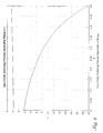
The curves of φ1,φ2,φ3 vs. r are shown in FIG. 2B.
The φ
1 and φ
3 curves have not extended to their asymptotic value π as it becomes numerically more and more difficult. Indeed, r=2 corresponds to p=2/{square root over (5)}˜0.8944 and r would increase more abruptly as p gets closer to 1 as
An artificial remedy is to set φ2 to 0 for r>1.5. The [φ1,φ2,φ3]−p subplot is given also to highlight this numerical difficulty.
The solution of (4.9) is a function of r which expectedly cannot be given as a closed form formula in terms of p and w. Nonetheless, by curve-fitting the solutions, the goal to achieve [x(t
3),y(t
3)]=[A,0] can be achieved.
The equation (4.14) terms are obtained by curve-fitting with respect to r<<1 (highly underdamped). To consider in addition the cases with r˜1 (moderately underdamped) and r>10 (slightly underdamped), (4.14) can be given in form of piecewise-defined functions for best quality of fit. Note that curve-fitting, if done properly, reduces the time/cost to recalculate new timings given a new p. For example, if the command input to the servo changes, the p and w values are placed in the equation (4.14) to generate new switching times.
Theorem 4.2. Consider (4.1). Then: For any 0≦p≦1, there exists a unique pair of switching times t1,t2>0 such that x(t)=A for all t≧t3=t1+t2 which is minimum time. Moreover, [t1,t2] can be given by the solution of the system (4.9), which can be solved from (4.11), whereas (4.14) provides approximations, as functions for r for t1,t2,t3, respectively.
Setting r=0, viz. p=0, results in
[cos φ3, sin φ3]=[2(cos φ2−1), 2 sin φ2]. (4.15)
Since |sin θ|≦1 and |cos θ|≦1, 0<φ
2≧{fraction (π/2)} and φ
1+φ
2≧π/2 follow, which further imply that
Hence, φ
1+φ
2≦cos
−1({square root over (3)}−2)=1.84206˜{fraction (7/12 )}π follows. The numbers given in (4.14) were obtained numerically, however. Those for φ
1 were taken by subtraction φ
3−φ
2. Note:
Note also that [φ1,φ2] exists for all r>0 and that there is no finite singularity in (4.10)-(411).
Elementary manipulations also yield
[cos φ1, sin φ1]=[2e rφ 3 (e −rφ 2 −cos φ2), 2e rφ 3 sin φ2], (4.16)
(4.10) and
The similarities in appearances between these and equations (4.8)-(4.10) include that they behave quasi-linearly or preserve some sort of symmetry. In fact, an equivalence of (4.10) reducing φ2 instead of φ3 is shown later.
Maximum-Amplitude Switching
FIG. 3 is a block diagram of an embodiment 300 of a servo system employing maximum amplitude switching as described in greater detail above. Servo system 300 comprises a switching element 302 and a servo 304. Switching element 302 accepts an input amplitude A, and outputs an amplitude to the servo 304. Switching element 302 includes a timer 306, and an inverter 308. The switching process of switching element 302 is pre-programmed with a maximum amplitude Amax for the particular servo 304 to which it is connected. The timer is coordinated to provide the output amplitude Amax to the servo 304 for a time period from 0 to time t1. At time t1, the timer switches the amplitude of the output to −Amax, and provides that amplitude −Amax to servo 304 for a time t2. In this embodiment, another switching is effected at a time t3=t1+t2. In this embodiment, the original command level amplitude A is passed to the servo 304 from time t3 onward. FIG. 10 shows an expected settling time for a servo system of this embodiment compared with other servo settling embodiments described herein. From FIG. 10, it is seen that improvement over unswitched serve systems is quite noticeable.
An embodiment of maximum amplitude switching process 350 is shown in FIG. 3A. Process 350 comprises determining a maximum input amplitude for a servo in block 352, determining first and second switching times in block 354, applying the maximum amplitude to the servo from time 0 to the first switching time in block 356, applying the negative maximum amplitude to the servo from the first switching time for the second switching time in block 358, and applying the command input amplitude from the second switching time forward in block 360.
The third switching process uses some extra degree of freedom, the resulting settling time is shorter than that from the input-parity switching process 250 described above.
Specifically, applying (4.1) with [A
1,t
1] followed by [−A
2,t
2] (A
1 and A
2 are not ‘related’ with the commanded constant input A), (4.6) still applies, while (4.7) becomes
and further, reduces to
e −rφ 3 [cos φ3, sin φ3]=[(1−μ)−(1+ρ)(1−e −rφ 2 cos φ2), (1+ρ)e −rφ 2 sin φ2] (4.19)
where
The rest of the work is similar to the solution process for the input parity switching case, except that the solution for [φ
1,φ
2,φ 3] will be a function of [A
1,A
2]. The resulting settling phase φ
3 is tabulated against A
1 and A
2 and the minimum is located; the minimizer [A
1*=A
2*] is
from which the name maximum amplitude switching is derived, which reduces (4.19) to
e −rφ 3 [cos φ3, sin φ3]=[(1−μ*)−2(1−e −rφ 2 cos φ2), 2e −rφ 2 sin φ2] (4.22)
(cf. (4.9)).
FIG. 3B plots [t
1,t
2,t
3] as a function of μ*. The characteristics of the switching times as functions of A/A
max as well as of p are quite linear.
where and are as given by the right-hand sides of (4.16). Note in particular, that there is a cross-over in t3 at μ*˜0.8, suggesting that employing a smaller ratio μ*>0.8 works better for larger p, and vice versa.
In comparison to the input-parity switching process 250, the switching phases now do depend upon A, or, more precisely, on the ratio μ*. Consequently, whenever a new commanded input arrives, the switching times are re-computed. This can certainly be made costless by using curve-fitting. The extra effort does offer shorter settling time. In fact, the maximum amplitude switching reduces the settling time by as much as 50% for μ*=½; for smaller A the settling time gets even smaller. This reduction proves very helpful for the servomechanism applied with multiple command inputs, i.e., a servomechanism in continuous operation.
While no attempt would be given to prove any optimality of (4.21), which applies to any A, it is worthwhile to point out its bang-bang nature. Note that as a common practice (at least in some bang-bang control texts), the ‘bang’ is often normalized with respect to the commanded input A. (Note that this, as a matter of fact, corresponds to the input-parity switching process.) As such, some better results may have been overlooked when there are more than one commanded input considered. However, the better results, if any, will readily fall from the application of the relevant equations and are within the scope of the present invention.
Turning-Points Input-Parity Switching
An alternative embodiment of the on-the-dot switchings described above, namely shrunk fit, input parity, and maximum amplitude switching, in which all the switching times are numerically obtained, is a slightly less analytical, closed-form switching scheme as described below. Select the switching times t1 and t2 as the first y-turning and x-turning times (from t1 onward).
When (4.1) attains its maximum velocity at t1, the ‘moment of inertia’ sustains and counters the new input −A for a certain period of time. The new input −A is injected so as to reduce the overshoot of (4.1). The velocity remains positive at this time. Switching the input parity to −A begins to reverse the ‘uphill’ trend to be ‘downhill,’ which needs to be reversed again at some time. A natural candidate for t2 is when (4.1) attains its (next) extremum x. The results of this switching process are analyzed below.
From (3.3),
from which cos φ=r sin φ at y′=0, viz.
[φ1 ,x 1 ,y 1 ]=[α,A(1−2pe −rα), Aωe −rα] (4.25)
where [x
1,y
1] becomes the initial condition for the second leg, i.e., (4.1) applied with −A. By replacing A with −A, from (3.27),
In this situation, a′>0 and b<0. Moreover, the situation here is different from solving for the excursion: A search is made for the very first phase φ
2 or time opportunity such that y=0 for the next switching, back to +A. By (4.7),
after algebraic manipulation. Thus, [x
3,0] is at hand to use Theorem 3.1. With ε
3=1−x
3/A=2−c′e
−rφ 2 ,
As a numerical example, with p=0.1 and σ=3, {overscore (t)}=1.471+0.422=1.892=0.6023π. Note that |ε3|<{overscore (ε)} in this case.
Any process involving a servo is amenable to the processes described herein. Thus, any second order servo application, such as tank turret control servos, angle to angle servos, targeting servos, and the like are applicable to the methods described herein.
On-the-Dot Switching With Non-Zero Initial Velocity
The above described embodiments have been analyzed with respect to an initial velocity of zero. However, in many situations, nonzero velocity is encountered in a switching process. For example, if a command is given to rotate a servo from a first angular position to a second angular position, and an intervening command is given to or received by the servo to move the servo to a third angular position before the servo has settled at the second angular position, it would be desirable to abort the command to move to the second angular position, and instead move directly toward the third angular position. However, in this situation, the servo is moving toward the second angular position, and therefore has an initial velocity which is not zero.
As noted previously, if the new servo command arrives prior to completion of a servo command (applying one the described switching process embodiments, for instance), a ‘hangover,’ remnant velocity will be the initial velocity for the new commanded input. If this remnant velocity is small, it can be taken as a perturbation. While applying the previous derived scheduling will witness some ripples, the switching process will still settle fast, as will be shown by simulation in the next section. A significant initial velocity is ensued, however, if the new command arrives abruptly. The scheduling of the switching process is therefore modified in another embodiment described below. The modification is sketched as follows.
Consider
x″+2pωx′+ω 2 x=ω 2 A, x(0)=0,x′(0)=y 0≠0. (5.1)
For the shrunk-fit switching process 150, the equations to be solved are
A 1[1−e −rφ(cos φ+(r−dη) sin φ), dωe −rφ(b cos φ+a sin φ)]=[A,0]. (5.2)
The second equation is solved for φ
1, substituted to the first equation, and solved for A
1. The solution of b cos φ+a sin φ=0 is now subject to a different requirement. Indeed,
which implies that necessarily, sin φ=b/c,−b/c if A1<A,A1>A, respectively. With the notation in (3.21), the following is obtained:
Theorem 5.1. (Shrunk-Fit Switching Process) For (5.1), the command schedule [φ
1,A
1] can be given either by
the latter applies provided that A<Amax (1−ce−r{overscore (β)}).
For the input-parity switching process, obtained in parallel to (4.5)-(4.6),
e −rφ 1 [a cos φ3 −b sin φ3 ,a sin φ3 +b cos φ 3]=[2(cos φ2 −e rφ 2 ), 2 sin φ2], (5.4)
from which
e −rφ 3 [a cos φ3 −b sin φ3 ,a sin φ3 +b cos φ 3]=[−2u,2ν] (5.5)
and then
where the ({circumflex over (·)})-notation is again employed in (3.21) with
Note that v→β (see (3.21)) as r→∞.
Moreover, the problem has now been complicated by η via {tilde over (ν)}: In comparison, μ the counterpart of ν or {tilde over (ν)}, rather, is definite because the sign of u is definite, while that of au−bv depends on η.
In parallel to (4.10),
More general but less conclusive, Lemma 5.1 below is the counterpart of Lemma 4.1.
Lemma 5.1. The following properties hold for the solution [φ
1,φ
2] of (5.5):
(b) 0<φ2≦π/2 if c≦2 (⇄ρ−≦η≦η+ (see (4.13)).
(c) There exist η
−<0 and η
0>η
+p>0 such that π/2<φ
3<π for
and no solution exists for η>η0.
(d) φ2→0 and φ1→{circumflex over (β)} as r→∞ if c<2.
Proof: For (a), from (5.6) and in parallel to (4.13)
If
whereas if
automatically, which leaves satisfaction of (5.10) to e
−rφ 2 >2/2+c only. For (b), consider
and recall Lemma 4.1(b). For (c), with φ2<π/ 2, a sin φ3+b cos φ3>0 and a cos φ3−b sin φ3>0. It is straightforward to see that if (a,b) has the sign combination (+,+), (+,−), or (−,+), respectively, φ3 must be in either first or second, either second or third, and either first or fourth. The ambivalences can then be reduced by virtue of continuity from the case with y0=0.
It is clear that while φ
1=0⇄φ
2=φ
3 has no solution by simply examining (4.8), a solution for (5.10) actually exists for a unique η>0. Indeed, by (5.10), (5.4) is reduced to
This, together with (5.3), leads to
It follows that b sin φ
2>0, reducing (5.11) to
and further to
and (5.12) to
2e rφ 2 ={square root over ((2−a)2 +b 2)}={square root over (1+2pη+η2)}. (5.14)
We thus have
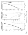
an equation in η. Evidently, Φ0.1(0)=−10ln2<0. By the facts that Φ0.1(0)Φ0.1(3.2)<0 and Φ0.1(−2)Φ0.1(−3)<0, solutions for Φp(η)=0 exist for 0<η<2 and −3<η<−2 for p=0.1, for instance. Via numerical (bi-section) search, the solution η of (5.15) is plotted in FIG. 4 as a function of p.
Note that η→±{square root over (3)} as p→0. Moreover, the obtained branches of solutions fit
[η+,η−]=[{square root over (3)}+151286p, {square root over (3)}e 5.25P], (5.16)
rather well. The [φ1,φ2,φ3]-curves, as η-parametric and p-parametric functions of p and of η are depicted in FIGS. 5 and 6, respectively. For comparison (and programming convenience, as well), the portions of curves which went beyond the interval in which φ1>0 are retained.
Note that for small y0, the switching phases are rather linear. The simple “linearity” may be useful for predicting/modifying the switching phases from those obtained for [x0,y0]=[0,0].
The analysis for input parity (250) and maximum amplitude (350) switching processes are shown in parallel below. The governing equation is a hybrid of equations (4.21) and (5.5):
e −rφ 3 [a 1 cos φ3 −b 1 sin φ3 , a 1 sin φ3 +b 1 cos φ3]=[(1−μ)−(1+ρ)u, (1+ρ)ν] (5.17)
where [ρ,μ] are as defined in (4.22), [u,ν] is as given in (4.13),
and [a
1,b
1]:=[1−pη
1,qη
1]. In parallel to those from (5.6) to (5.15),
where
and it follows that
While the described embodiments have been discussed with respect to underdamped servo systems, the principles apply as well to embodiments having overdamped systems where p>1. When the servo is unstable, but has real eigenvalues, no solutions to the timing equations exist. However, in certain situations of unstable servos, where the instability meets certain conditions, solutions still exist for the timing equations. For example, if the eigenvalues of a servo are complex conjugates, solutions exist whether the servo is unstable or not. In essence, if the damping ratio p of an unstable servo meets the condition 0>p>−1, then the servo, while unstable, is not too unstable to solve, and solutions exist. For damping ratios of p<−1, no solutions exist.
In these embodiments, the overdamped counterpart of (4.1) and §4 becomes:
x″+2pωx′+ω 2 x=ω 2 A, p>1 and [x,x′]=[0,0]. (6.1)
It should be understood that such analysis also applies to nonzero initial velocity, as one of skill in the art would readily observe.
Denote by [q,r,φ,φ1]:=[{square root over (p2−1)},p/q,qωt,qωt i]. Then the two associated characteristic roots are given by
[s 1 ,s 2 ]=−qω[r−1,r+1] (6.2)
Setting x=c
1e
s 1 t+c
2e
s 2 t+A so that y=x′=c
1s
1e
s 1 t+c
2s
2e
s 2 t, and solving for c
1, C
2 and then for x,y as
If x0=0, y0=0, (6.3)-(6.4) reduce to
[x,y]=[A{1−½[(1+r)e −(r−1)φ+(1−r)e −1r+1)φ], ½qω[e −(r−1)φ −e −(r+1)φ]]. (6.5)
Natural Settling Time
While knowing x<A (assuming A>0), there appears no simple, analytical way to find settling time via solving min φ>0 from the defining inequality
By numerical search and curve-fitting (with a trivial range of deviation), however, the settling time (normalized by ω=1) as a function of p and {overscore (ε)} is obtained:
The settling time is nearly linear in p.
For (numerical) examples, {overscore (ε)}=5%,
p=1.1 1.2 1.3 1.4 15 1.6 1.7 1.8 1.9 2.0 2.1 2.2 2.3 2.4
t=5.47 6.19 6.89 757 8.24 8.89 953 10.17 10.81 11.44 12.06 12.69 13.31 13.93 and for p=2,
{overscore (ε)}=1% 2% 3% 4% 5% 6% 7% 8% 9% 10%
{overscore (t)}=17.44 14.85 13.34 12.27 1 1.44 10.76 10.18 9.69 9.25 8.85.
Settling Time With Switching
Observe first that e−(r−1)φ−e−(r+1)φ≠0 for all t>0, i.e., there exist no x- nor y-turning points if |p|>1. As such, for one thing the Shrunk-Fit switching process 150 does not apply to any real-mode case. Note also that A1=A under process 150 (even with approximation).
The following considers the input-parity switching process 250 for (6.1), by applying switching commands [+A1;t1;−A2,t2;A,t] for maximum amplitude switching study, and then by reducing the results to the input-parity case. By (6.5),
[x 1 ,y 1 ]=A 1[1−½((1+r)e −(r−1)φ 1 +(1−r)e −(r+1)φ 1 ),½qω(e −(r−1)φ 1 −e −(r+1)φ 1 )] (6.8)
immediately. It follows that
Thus, with algebra,
the following are readily obtained
Evidently, having y2=0 is equivalent to having
[(1+ρ)−e −(r−1)φ 1 ]e −(r−1)φ 2 =[(1=ρ)−e −(r+1)φ 1 ]e −(r+1)φ 2 =:χ<1+ρ. (6.12)
From (6.12), solve for φ
2 as
Furthermore, (6.12) also reduces x
2=½(1+r)A
1χ+½(1−r)A
1χ−A
2=A to χ=μ+ρ. By back substitution of (6.13) to (6.12),
To solve (6.14), it is more convenient to consider
It is then straightforward to obtain
That is, F(·) is strictly increasing. Hence, a solution φ
1>0 exists if and only if F(0)F(∞)<0 viz.
which is trivially the case if and only if
0<μ<1 and 0<ρ≦1. (6.18)
With the input-
parity switching process 250, A=A
1=A
2, ρ=1, μ=1, χ=2 trivially and (6.13)-(6.14) reduce to
In spite of their simple appearances, the fact that F(∞)=0 indicates that φ1=∞ is the only solution, which is useless. As such, there exists no input-parity switching process solution for (6.1).
In comparison, the maximum-
amplitude switching process 350 entails ρ=1 only. Thus, (6.19) still applies, whereas (6.14) becomes
In the previous notation (6.15),
A finite φ1>0 exists. The solution curves of [t1,t2,t3] as parametric functions of ρ=1, μ and p are shown in FIG. 7.
While it might appear acceptable to have approximity instead of strict equality in (6.20) for input-parity consideration (now that +∞ is the only exact solution), it turns out that input parity switching offers little in this case, since the trajectories of the natural and the switched servos are almost identical.
Consider now the degenerate case that p=1, a critically damped system, resulting in r=−ω a double root. Formulating x=e−φ(c1+c2t)+A so that y=e−φ[−ωc1+c2(1−φ)], and solving for c1 and c2:
x=e−φ{(x0 −A)+[y 0+ω(x 0 −A)]t}+A, (6.22)
y=e −φ{−ω(x 0 −A)+[y0+ω(x 0 −A)](1−φ)}, (6.23)
which reduce to
[x,y]=[A[1−e −φ(1+φ)], Aωφe −φ] (6.24)
for x0=0 and y0=0. Again, the shrunk fit switching process 150 has no solution.
For the input parity switching process
250, observe that
By setting y
2=0,
and by setting x
2=A and simplifying,
is obtained.
By the facts that F(0)=ln[ρ/(μ+ρ)]<0, F(∞)=ln[(1+ρ)/(μ+ρ)]>0 if 0<μ<1 and
a solution φ1>0 exists, as well.
For p<−p1, (6.12) applies still, with −(r−1)>−(r+1)>0. It follows that 1+ρ−e−(r−1)φ 1 and 1+ρ−e−(r+1)φ 1 must necessarily have the same sign. As either possibility fails (6.13), for p<−1, this switching process does not apply. This holds for any ρ, including that for maximum-amplitude switching ρ=1.
For p=−1, it suffices to reverse signs of certain terms in (6.21)-(6.27), yielding
The equation for φ
1 then becomes
which is impossible since φ1>0.
As is evidenced by reading out from FIG. 8, there exists a minimax for μ=0.8 (by taking μ as a parameter); it has appeared that this might be true for all ρ. Recall from FIG. 3B that this ‘minimax’ also exists for 0<p<1. This was not exhibited in FIG. 6.1 (p>1), however.
Derivation of the curve-fit results parallel to (4.23) for p≧1 and the results for the cases with nonzero initial velocity parallel to §5 are within the scope of one of skill in the art, and are within the scope of the present invention.
Some Operational Considerations
Servos are often used in continuous mode, that is, the servos receive commands one after the other in a continuous fashion. Further, some servos have command structures with quantized levels for the command, that is, there are specific quantized levels at which the commands are available, instead of along a continuous spectrum of levels. The various embodiments of the present invention as described above are applicable to such servos and to such command level structures.
In this section, considerations are given to two issues that arise naturally in putting the results to practical use. One addresses using the servos in continuous operation, i.e., the servos receiving commands one after another. The other, implicitly related to the first, is concerned with having not analog but quantized levels of command available to the servos.
As indicated in equations (3.16)-(3.18), solutions of the right switching phases (times) can be given by preparing off-line formulae derived via curve-fitting and by retrieving their values in on-line operation mode. A small block of memory is needed to store the coefficients pertinent to the retrieval. It is, however, feasible as well that the right switching phases be solved on-the-fly as the solutions converge rather quickly even in the maximum amplitude switching process 350 for which the timing needs to be re-computed upon arrival of new command.
Continuous Operation
The above switching schemes work well if the servomechanism is given with one command level A. In addition, some degree of robustness of the system given variations in mass, viscosity, stiffness, initial position and velocity, and the like is also present. In a situation in which a servo expects more than one commanded input constant, the following applies:
Consider the following servo input:
Furthermore, assume that as t=0, x(0)=0 has been ensured (by initial pre-operation calibration). Then, as long as
t 3 <t 1 <t 2 −t 1 <t 3 −t 2< (7.2)
and as long as the new command input is ‘reset’ by having
A 1 =A 1, A2 =A 2 −A 1 , A 3 =A 3 −A 2, . . . , (7.3)
the switching scheme operates as expected.
If the new command arrives too early and is in the reverse direction of the last leg (resumption) of switching, there will be a nontrivial delay before the new command is well served. To reduce this delay, in one embodiment the timing for the switching is reset (instead of letting it run thru its course) whenever a new command arrives, regardless whether the previous command has been fulfilled. Consider the scenario that τk+1<t1,
τk :=t k+1 −t k.
In this situation, a new command arrives while (3.1) is at its normal phase even before reaching the first switching. Thus, [x(τk),y(τk)], and upon reset [0,y(τk)] is the initial condition associated with (3.1) in applying the various embodiments of the switching schemes to serve the command Ak+1−Ak. Assuming that a measurement x(τk) is not available, x(τk) will be somewhere between 0 and Ak−Ak−1, its previous goal. This scenario has, in fact, motivated the need to look for an algorithm with which the settling time could be further shortened so as to accommodate frequent changes of command levels.
As mentioned earlier, by applying the convolution theorem the results may apply to serve with a more sophisticated command set; therefore, the discussion focused on piecewise constant commands is not a restriction but rather a simplification. Indeed, if the actuator has a much faster natural frequency than the servo command set has, piecewise constant commands serve well as an approximation.
Quantized Levels of Command
Let Â:={A1,A2, . . . ,AN} be the quantized levels of command a servomechanism is able to generate (besides zero), 0<Ai in ascending order, and let AN>A ∉ Â be the input level commanded. Consider the following question:
It is possible to schedule the input command levels such that x(t) is settled nearest to A. For example, when only discretized responses can be generated by the actuator employed, e.g., step motors, on-off valves, etc., a solution is given below.
For simplicity, consider first that A1=A2−A1=A3−A2= . . . =AN−AN−1, i.e., uniformly spaced. Let
A k:=mink {|A−A 1|, . . . ,|A−A N|}, (7.4)
i.e., A rounded off to its nearest quantum Ak. Apply the maximum amplitude switching process 350 first with Ak, viz. +AN for t1(Ak,AN), then −AN for t2(Ak,AN). Now, at t3=t1+t2, if Ak is applied, x(t)=Ak for t≧t3, and thus there is a steady-state error
|A−A k|≦½A 1 (7.5)
which is a minimum possible but unavoidable. Note that Ak−1 or Ak+1 may substitute for Ak if there is any additional constraint on the steady-state error. Note also that only one maximum amplitude switching is needed and the settling time incurred would be this t3 only.
Consider next the case that the input levels are not uniformly spaced. Now, apply maximum amplitude switching with At 1 for any At 1 <A first. Apply next with
A t i <A−A t i−1 , i=2, . . . , m (7.6)
until the steady-state error is acceptably small. By (4.31), it is not difficult to see that the total amount of settling time is given by
For instance, m=2, which hopefully would be the typical case,
This embodiment shows that it is possible to alleviate the problem of inadequate performance in resolution due to having large quantized error by switching.
Simulation Results
Various simulation results for the embodiments presented above are shown in graph form in FIGS. 9 to 17. The figures have been discussed or mentioned briefly above in terms of actual processes such as shrunk fit process 150, input parity process 250, and maximum amplitude process 350. FIG. 9 shows performance comparison of a natural, that is unswitched, servo versus a servo switched using input parity switching process 200. Lines 902 and 904 represent unswitched position and unswitched velocity, respectively. In this embodiment, the command level is 10. Lines 906 and 908 represent switched position and switched velocity, respectively.
FIG. 10 shows position comparisons for unswitched servo (line 1002), servo switched with shrunk fit switching process 100 (line 1004), servo switched with input parity switching process 200 (line 1006), and servo switched with maximum amplitude switching process 300 (line 1008).
FIG. 11 shows position trajectory curves for an input parity switched process 200 with a range of initial nonzero velocities.
FIG. 12 shows position and velocity trajectory plots for an unswitched servo ( lines 1202 and 1204 respectively) and for a maximum amplitude switching process 300 ( lines 1206 and 1208 respectively), when the servo is overdamped.
FIG. 13 shows position and velocity trajectory plots for an unswitched servo ( lines 1302 and 1304 respectively) and for a maximum amplitude switching process 300 ( lines 1306 and 1308 respectively), when the servo is critically damped.
FIG. 14 shows an unswitched position trajectory plot for an unstable system (line 1402) versus a maximum amplitude switching process 300 position trajectory plot for the unstable system (line 1404) for a command level of 10.
FIG. 15 shows a graph of a series of command levels 3, 6, −1, and 1, as well as position trajectory plots for an unswitched servo (line 1502) and for a maximum amplitude switching process 300 servo (line 1504).
FIG. 16 shows a graph of a trajectory plot for a servo using quantized servo commands and maximum amplitude switching process 300. The desired command level is approximately 7.7. The nearest switching levels for servo commands are 7 and 8. This embodiment uses a defined duty cycle to alternate between allowable levels 7 and 8 such that the position is in proportion to the actual command.
FIG. 17 shows a graph of various position trajectories for unswitched servos (line 1702), and for switched servos using one of the described switching processes 100, 200, or 300 for timing errors of 5% (line 1704) and 10% (line 1706). In other words, the switching times are off by the factors of 5% or 10% due to some error, such as imperfect curve fitting, changing commands, and the like.
CONCLUSION
Analysis and simulation results have been given to three switching processes, namely shrunk fit switching, input parity switching, and maximum amplitude switching. These switching processes, and the apparatuses that embody the processes, achieve quick settling and trivial overshoot for second-order LTI servomechanisms. The switching processes achieve the results without the use of sensors.
The embodiments of the present invention are applicable not only for underdamped servos, but also to certain zero-damped, overdamped, critically-damped, and oscillatorily-unstable servos. In addition to these, the processes are applicable to underdamped servos with a nonzero initial velocity.
Application of the processes to time-continuous operation of servos and to servos that are equipped only by quantized command level is also embodied.
In the embodiments, no sensors are used to determine position of any servo mechanism. Since sensors are not required, numerous advantages accrue. Among the advantages of sensor-free servo settling systems such as those described herein are increased payload availability, reduced weight, reduced size, and the like.
In specific embodiments, methods for controlling a servo of any order include at least re-scheduling of a servo input command signal by applying a switching schedule consisting of a sequence of switching instructions such as amplitude-timelapse pairs, to the servo, and returning to the original servo command at the end of the calculated switching command schedule.
In another embodiment, a switching process-controlled servo control system, as stated above, includes a servomechanism, a processor operatively connected to control the servo, and a timer programmed to apply input command signal amplitudes at pre-determined switching time instants.
In yet another embodiment, a command program for controlling a servo without using sensors includes machine-readable instructions for effecting the method of controlling a servo by applying switching command schedule calculated as stated above.
In still another embodiment, a method of controlling servos of the second order includes formulating the two algebraic conditions that equate the velocity to zero and the position to what originally commanded, at the end of the switching time schedule.
In still another embodiment, an algorithm for programming the instructions includes effecting switching process-controlled servos by curve-fitting the solutions of the algebraic position-velocity equations for efficient execution of the switching program.
Three different implementations of the methods stated above, to meet differing performance-cost specifications, are supplied. The first implementation requires one switching instruction, the amplitude of which is a calculated proportion of the original servo input, and the timelapse of which phases exactly half a cycle from commencement. The second implementation settles faster than the first but requires two switching amplitude-timelapse instructions, the first amplitude of the two being the same as the original servo input, and the second, the negative of the first, and the two timelapses being specified by the unique solutions of the two algebraic position-velocity equations. The third implementation settles the fastest of the three, and requires two switching instructions as well, of which the amplitudes are the maximum and its negative that the servomechanism can provide, and the two timelapses are specified also from the corresponding position-velocity equations.
Application of the various embodiments of the present invention can be made to numerous systems, including by way of example only and not by way of limitation any positional and rotary platforms upon which the servos operate, such as jet reaction control systems, fire control systems, hard disk drive control systems, low-cost guidance systems, numerical precision control systems, elevator debouncing control, tracking radar, auto pilot, hard disk read/write head movement control, scenery changes in virtual reality environment, helmet-mounted displays, and the like.
All the timing for the switching embodiments described herein can be obtained on an off-line basis via curve-fitting, which is helpful for practical servo application.
Embodiments for overdamped systems, critically-damped, and, in fact, systems with unstable complex modes are also presented. Furthermore, some aspects of applying these switching processes in practical, that only discrete/quantized levels of inputs available, are elaborated as well.
Also, making use of the convolution theorem, the processes and apparatuses of the various embodiments of the present invention are extendable to accommodating a larger class of non-constant servo commands.
It is to be understood that the above description is intended to be illustrative, and not restrictive. Many other embodiments will be apparent to those of skill in the art upon reading and understanding the above description. The scope of the invention should, therefore, be determined with reference to the appended claims, along with the full scope of equivalents to which such claims are entitled.